In this brief review, I will talk about Exploratory Desktop, a fresh approach to building visual analytics and interactive dashboard. If you happen to be one of those cool kids who swear by dplyr, pipe & co, this cool app is worth a look, even if, well, we can’t do data science in a GUI.

I have been following the development of Exploratory since its inception, or when the very first beta was released. It is continuously updated and it has smoothly evolved toward a full-featured UI for exploratory and, more recently, explanatory data analysis. For the latest news (version 4.2), see the blog post from Exploratory team. Kan Nishida, the founder of Exploratory, is regularly posting tutorials and hot release news on Medium.

At its heart, there is the open-source R statistical software and the tidyverse ecosystem. The original idea of Exploratory is to propose a clean UI that allows to transparently use most of the tidyverse packages through analytical steps that can be chained together, much like in Knime or Rapidminer. Although I never really used this app in my previous work, I suggested to some students interested in an alternative approach to data science with R (read, without the command-line stuff) to take a look at it, just in case they would find it more convenient than RStudio or other IDEs.

When you first launch Exploratory, it will install the latest R release and around 170 required packages. Everything goes under your home directory (~/.exploratory on my Mac) so that it does not interfere with existing installation of R or related packages. Beware that it amounts to around 1.3 Go in your home directory (+ 650 Mo in your /Applications folder).

Let’s get started: importing some data

I have tried the hard way but it was too much a pain for this short review. See the sidenote.

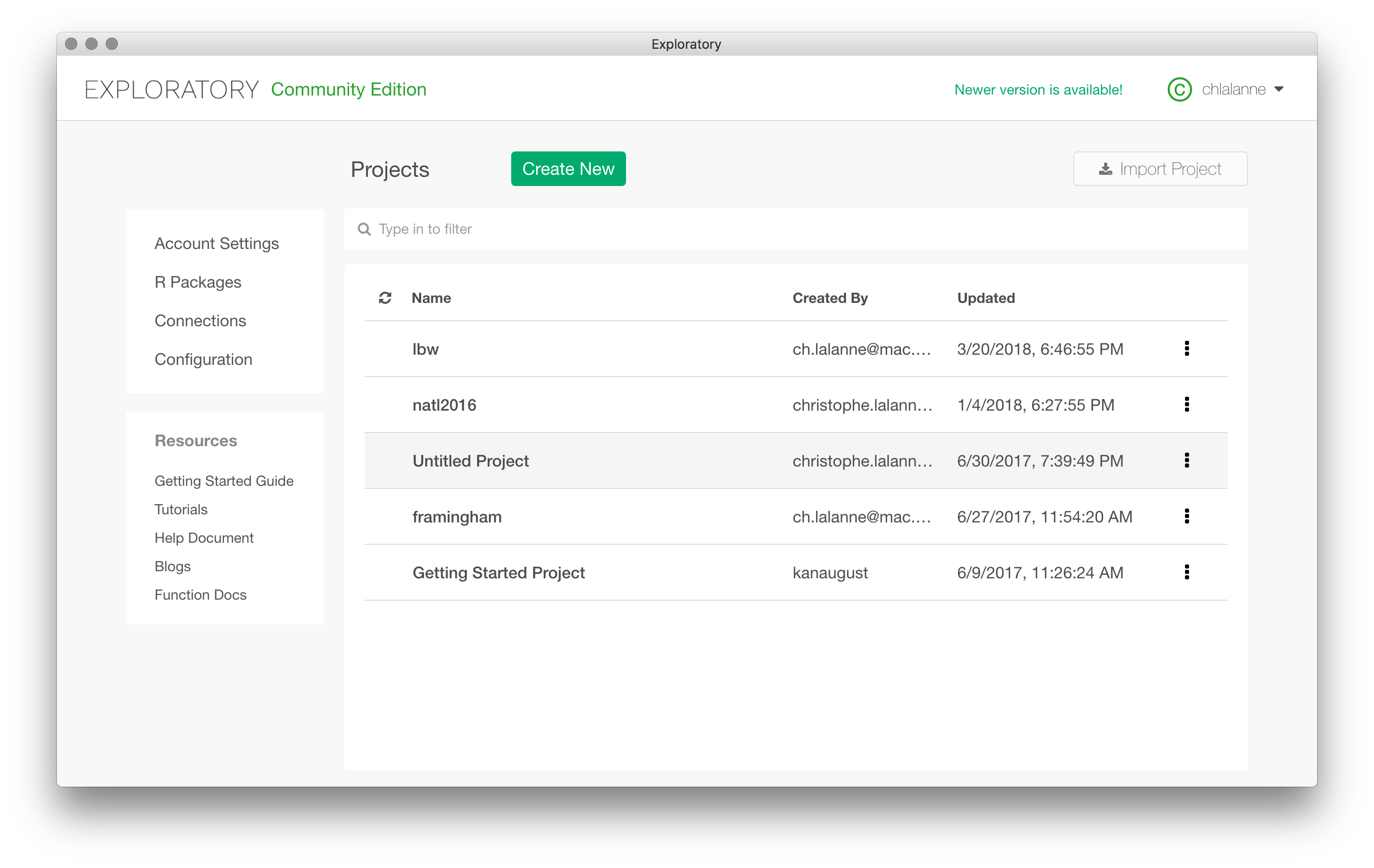
So I will stick with the birth weight dataset from Hosmer and Lemeshow that I have been perusing for my courses the last 10 years or so. Let start a new project and import a dataset as a CSV file. You can also import the RData file that comes with R in the MASS package (birthwt). Once it is done, the project will be listed on the welcome screen.

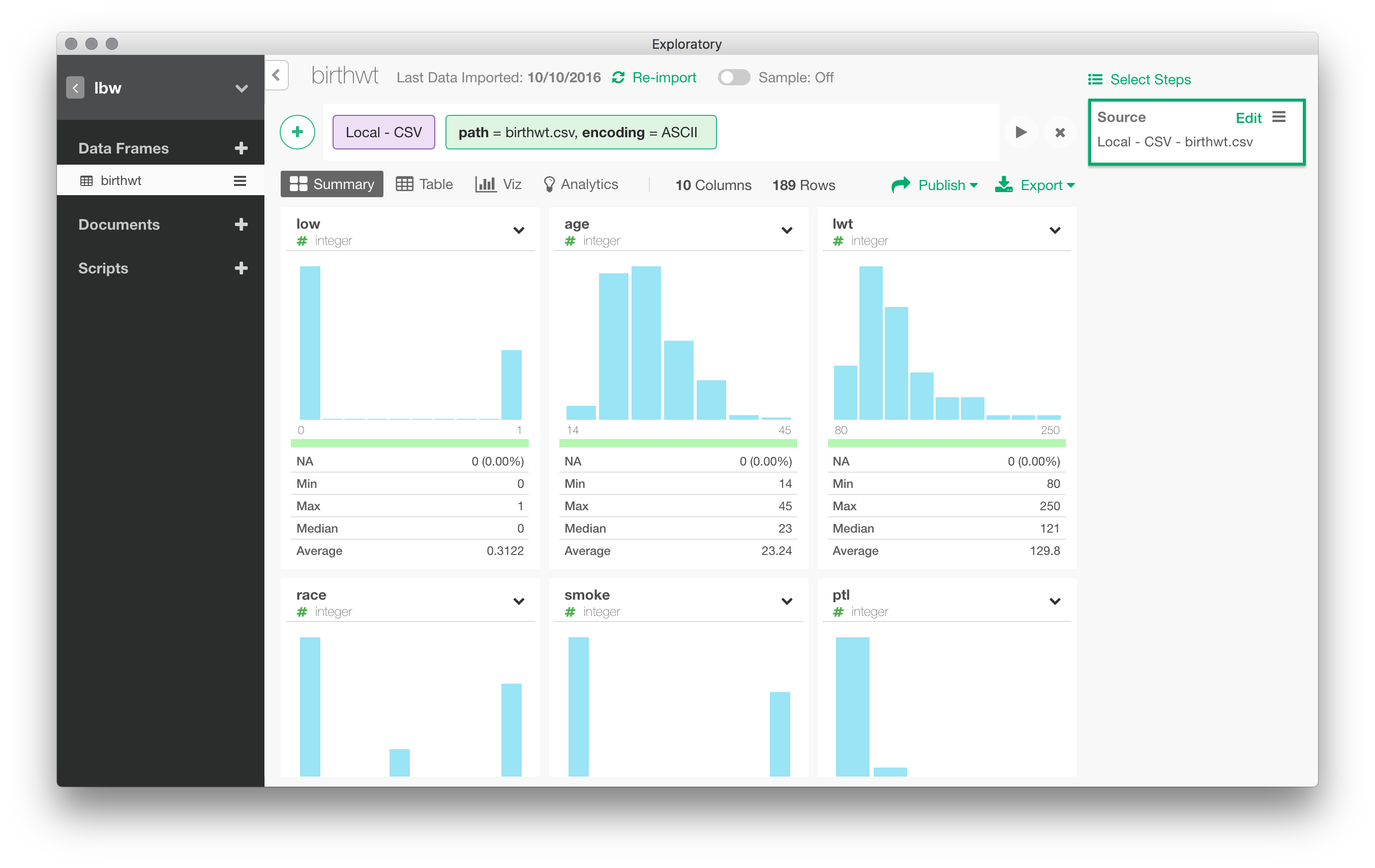
Once the data are imported in Exploratory, you are presented with a summary view, sort of a visual dashboard of all variables available in the local data frame. I like the idea. It has been removed in a previous version of Exploratory, but it is back again. Although it takes a lot of space on screen, I really think it is a good idea to summarize each variable using visual information.

Data munging

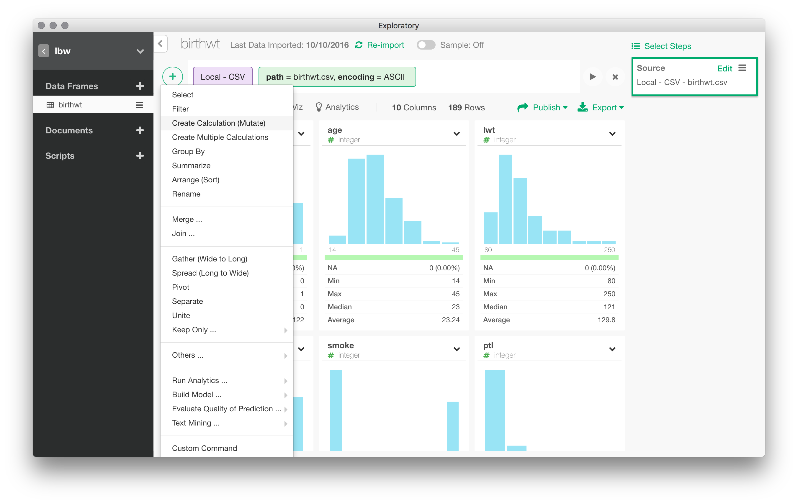
You have probably noticed the big “+” icon on the top menu bar. “The “+” sign stands for the main “Actions” menu. It allows to create a new action on the active dataset, e.g., operate on an existing variable or apply a group-wise operation on the full dataset. Actions are recorded as (analytical) steps in Exploratory Desktop, and they are displayed on the right vertical panel.

As discussed above, Exploratory is built around the dplyr package, so don’t be surprised if you find a lot of commands that are used in any dplyr tutorial. Recall that dplyr is basically organized around group_by() (to split data by group(s)), summarise() (to aggregate data), mutate() (to transform variable inline), filter() (to select observations/rows in a data table), select()(to select variables/columns), arrange() (to order variables/columns).

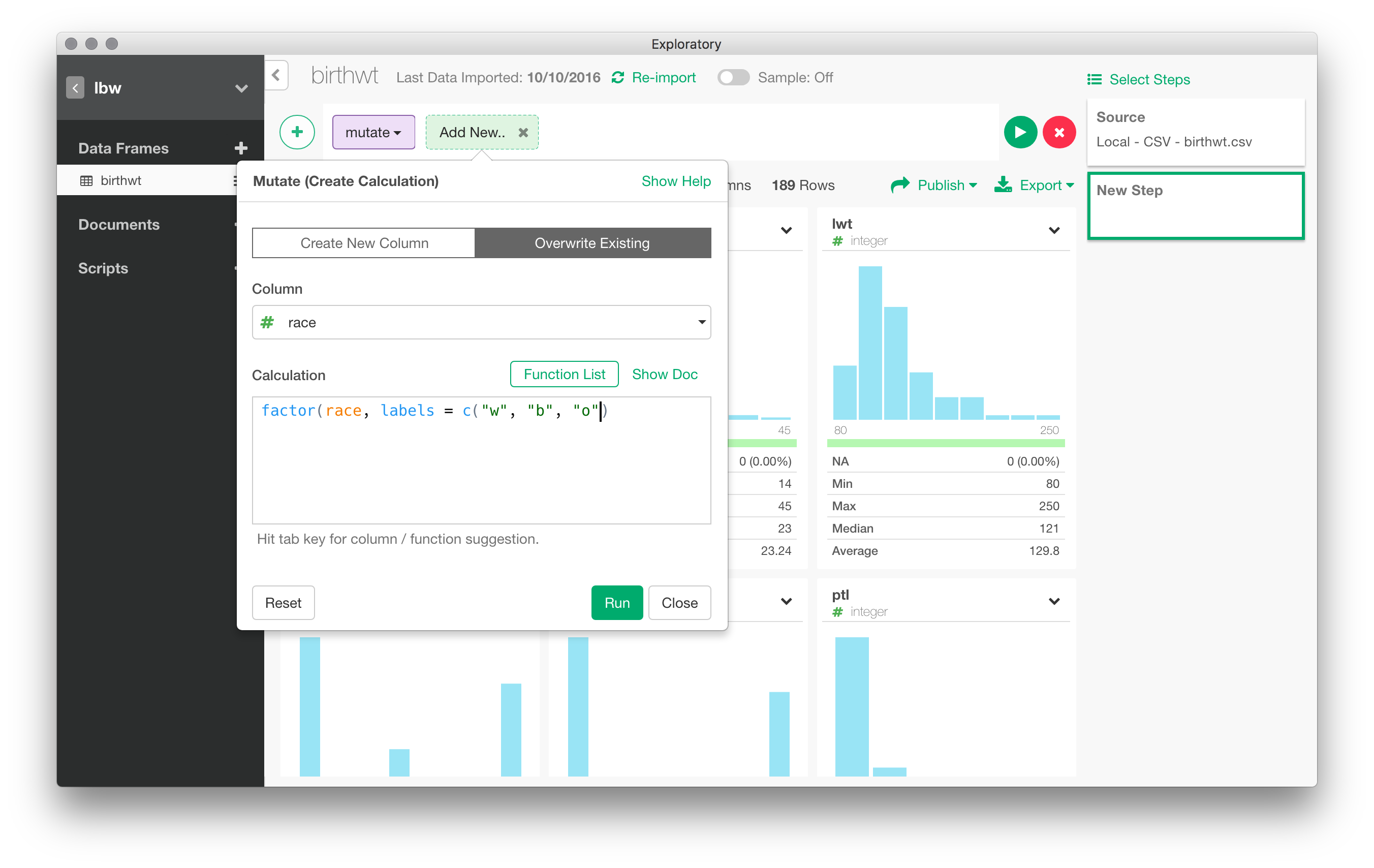
For instance, the race variable is treated as a numeric variable. To recode race into a factor, we can navigate through the Actions menu and choose “Mutate”. Without surprise, this relies on dplyr::mutate() and allows to transform variable inline.

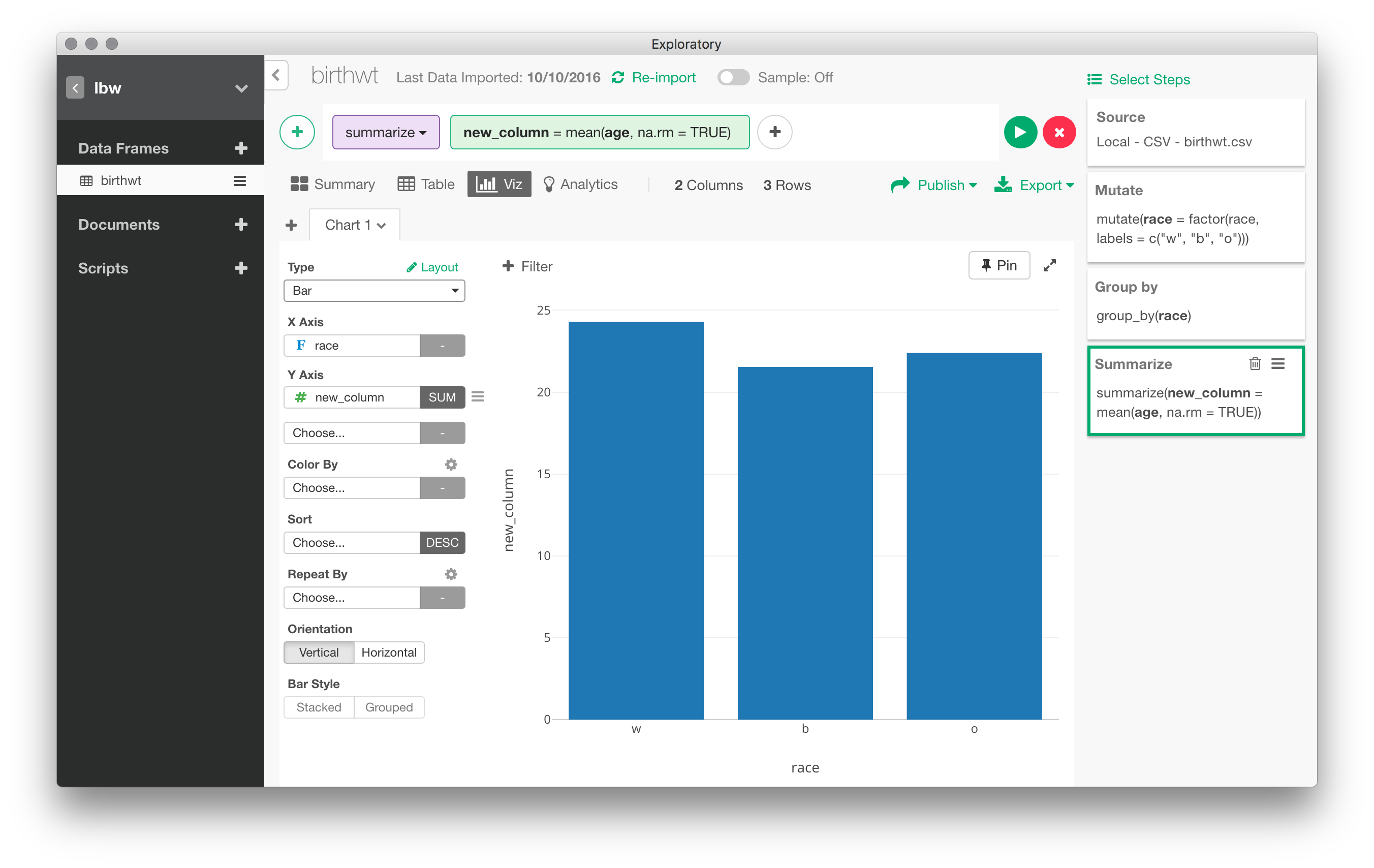
You can aggregate data in multiple ways: pivot table, conditional means, counts of levels of a factor, etc. For example, we could easily compute the mean of bwt by values of race. Every action results can generally be represented graphically. Here, with the preceding example, we can go right to “Viz” panel and the default is a bar chart for the three means. Note that several options are available that allow to customize the default rendering, including axis annotation, creating small multiples through the use of one or more “facets”, and so on.

Statistical modeling

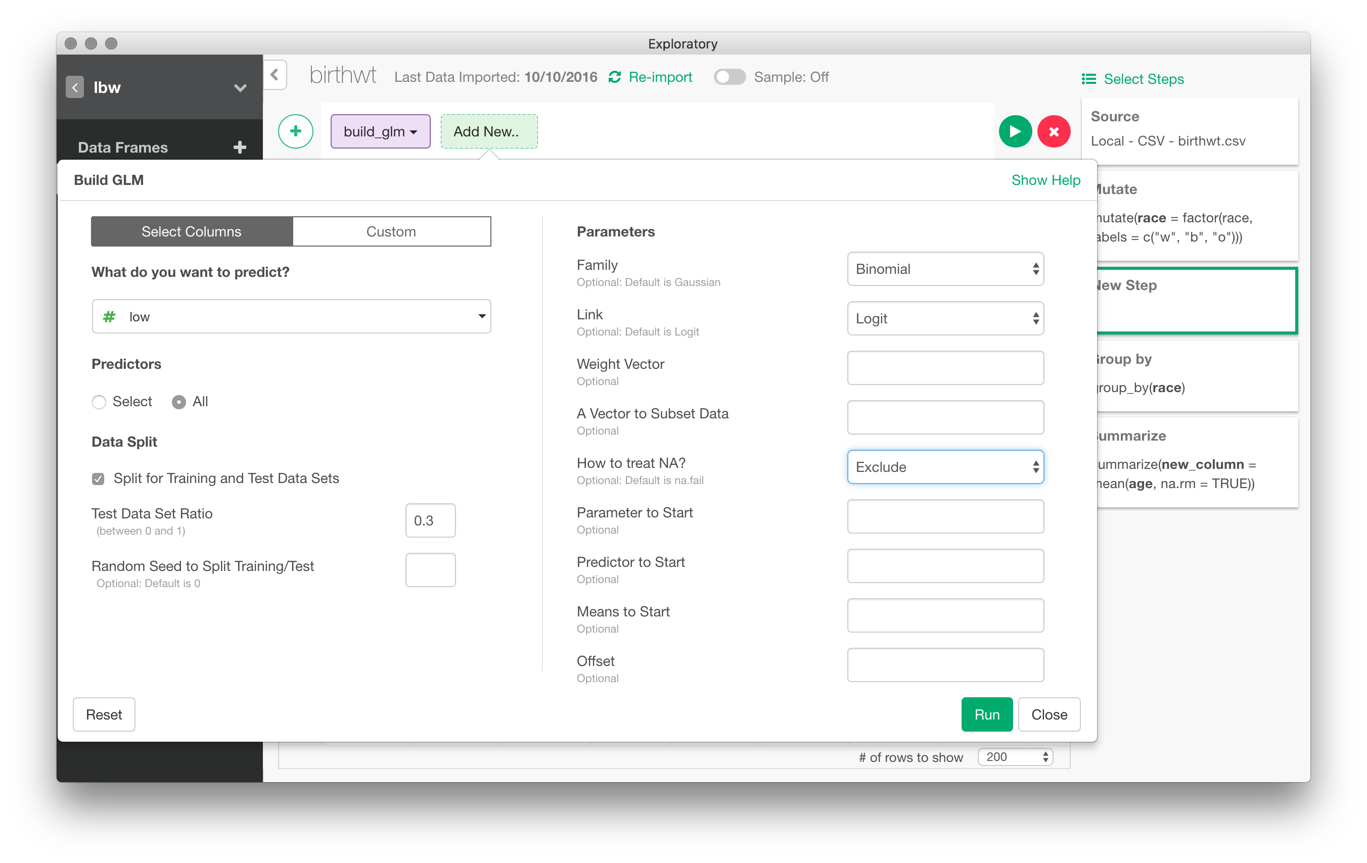
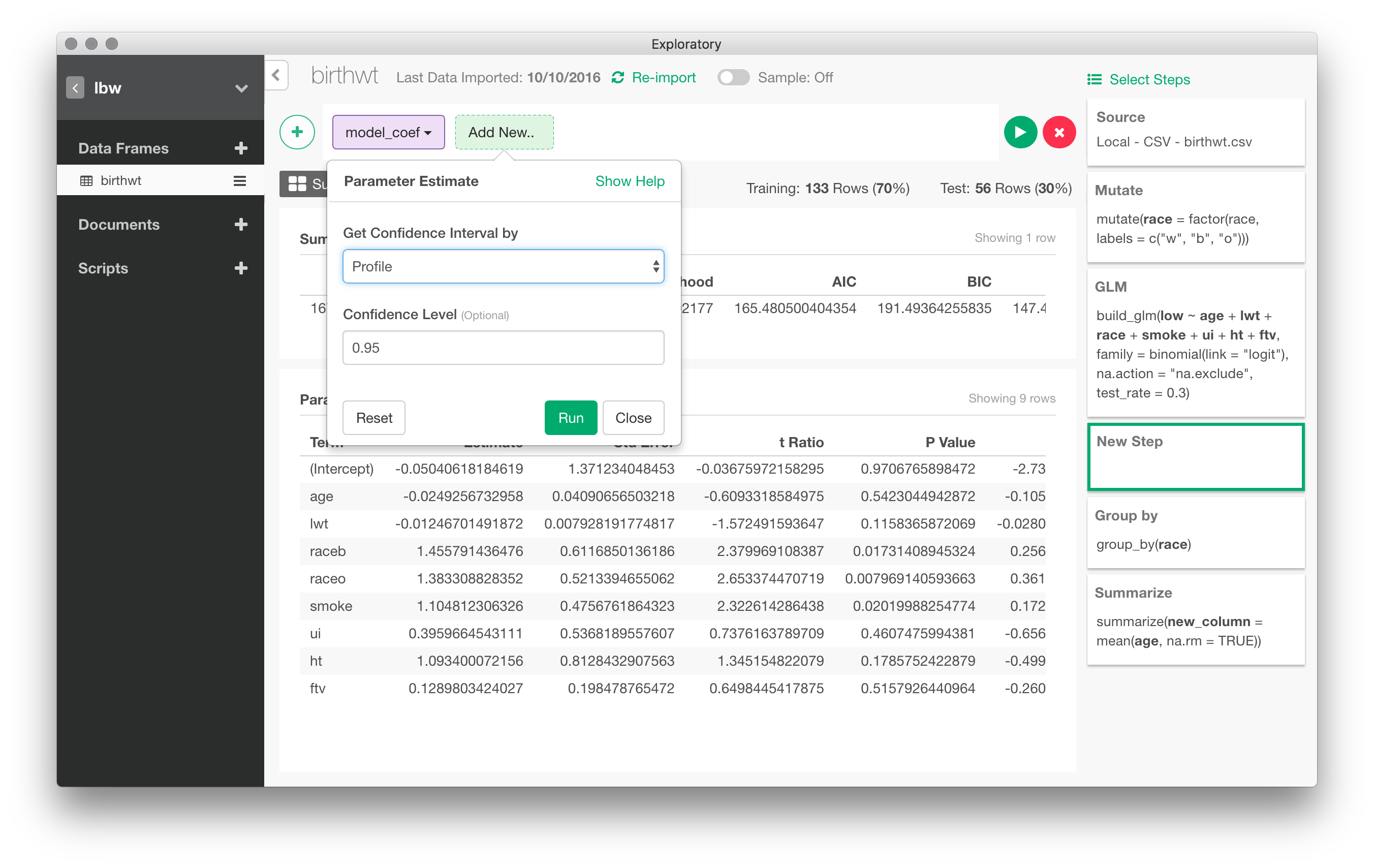
In the following picture, I have set up a logistic regression to predict low birth weight depending on values of all other variables (I skipped the bwt varible afterwards)

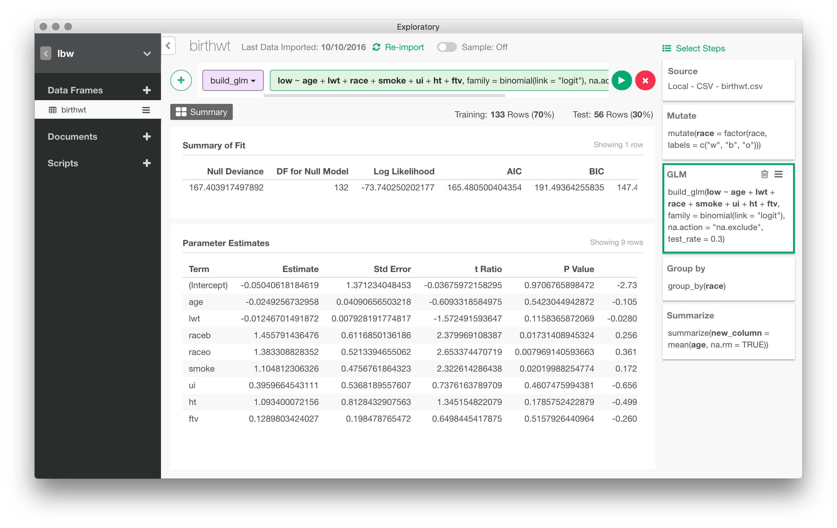
Here are the results for the basic model (with a 30% holdout sample). Confidence intervals are readily available in a post-processing step:

Beside linear regression and the GLM, there are a few other models available at the time of this writing, namely Extreme Gradient Boosting, Random Forest or Survival Cox regression. There are also dedicated modules for text mining, geospatial data visualization and time series forecasting (using the Prophet algorithm).

I should note that it is also possible to add custom notes to each analytical steps, and to record the results in a separate Markdown report file.

Conclusion

That’s it! If you want to try Exploratory Desktop, no regret, just do it. I am more of an ESS guy, so I always have a hard time staying focused in a graphical user interface that soon or later call for custom user scripts or the use of external command-line tools. Hopefully, Exploratory allows to write R scripts directly instead of relying entorely on the menu driven UI. There is good support for data import/export and database connectors are ok as long as you don’t have to work with esoteric NoSQL backends. The ability to process GeoJSON data is a plus, as well. I never understood why this app has not (yet) get the credit it surely deserves.

Sidenote

Exploratory Desktop does not play well with large datasets, at least when it comes to import 3 Go CSV files. For instance, I initially planned to use the following dataset for the above illustrations but had to stay with a modest one because of large memory overload. Here is how I started this review (very) long ago.

The data used throughout this review were fetched from the National Bureau of Economic Research (NBER) but are otherwise available on the CDC portal. They are available in CSV or Stata format. Note that the CSV file is 2.2 Gb and contains 3,956,113 records. The Stata file is more convenient since variables are already labelled and in the right format. It is as easy to import a delimited text file than proprietary formats like Stata or SAS, thanks to the haven package. It took about 2-3 min to preview and load the data in Exploratory on a Macbook Retina 12” running High Sierra with 8 Gb RAM (the process eats up all my RAM due to other applications running in the background, though).

Here are some benchmarks using more (compared to base R read.csv() function) or less (default options for data.table and readr were used) efficient approaches to load the data in CSV format right into R:

• data.table::fread() takes 56 sec; object.size() gives me 4512.4 Mb
• readr::read_csv() takes 193 sec; object.size() gives me 4784.1 Mb

(Python pandas.read_csv() is a winner of a little on that one with 163 sec.)

In comparison, loading the Stata file in Stata is almost instantaneous. Since Exploratory also accepts database connection, we could load the data into a dedicated PostgreSQL table and work from there. There are various ways to import CVS data into SQL. One approach is to use COPY (and I believe it is the faster option in our case), another approach relies on Python with, e.g., csvsql from csvkit or Pandas’s to_sql() utility. Yet another way is to use pgloader. Pure PostgreSQL solution require that we provide field specificatons (name and storage mode) for the table. Fortunately, the NBER provides a Stata dictionary that can be used to fill out the required information, pending some minor formatting issues that were handled using Perl.

To sum up, a straightforward technique from a Terminal is to use “csvkit” command-line tools:

$ createdb natl2016
$ csvsql --db postgresql://5432/chl --table natl2016 --insert natl2016.csv

Using “pgloader”, it should not be too hard to populate a PostgreSQL table using a custom command file. I should also note that it is possible to work on a sample of the dataset, which is what we will do next.