Some notes I took during the 31th ISBC conference. I only attended the first two days, with sessions mostly oriented toward genetic epidemiology. An extra session around latent variable modeling was also present. This gives me the opportunity to summarize two aspects of statistical modeling that I actually like a lot, namely biometrics and psychometrics.

The sequential rejection principle of family-wise error control (A. Solari)

In the context of GWAS, where we usually work with 500,000 SNPs or more, and where each SNP represents one hypothesis to test, the nominal p-value would have to be set to 1e-7. Even if SNPs are grouped by chromosomal region, we still have very low p-value (p < 𝛂 / # regions tested). There is thus a compromise between an increase in power (by working at a higher level than single unit, e.g., region or chromosome) and an increase in statement. However, the problem with region-based testing is that if H0 is to be rejected, we cannot say in turn which of its SNP(s) is/are implicated in the uncovered association.

There comes graph-structured hypothesis, whereby hypotheses are arranged in a tree structure based on (1) prior biological knowledge (Fig 1a), (2) logical relationship (Fig 1b), or (3) a data driven principle (e.g. linkage disequilibrium).

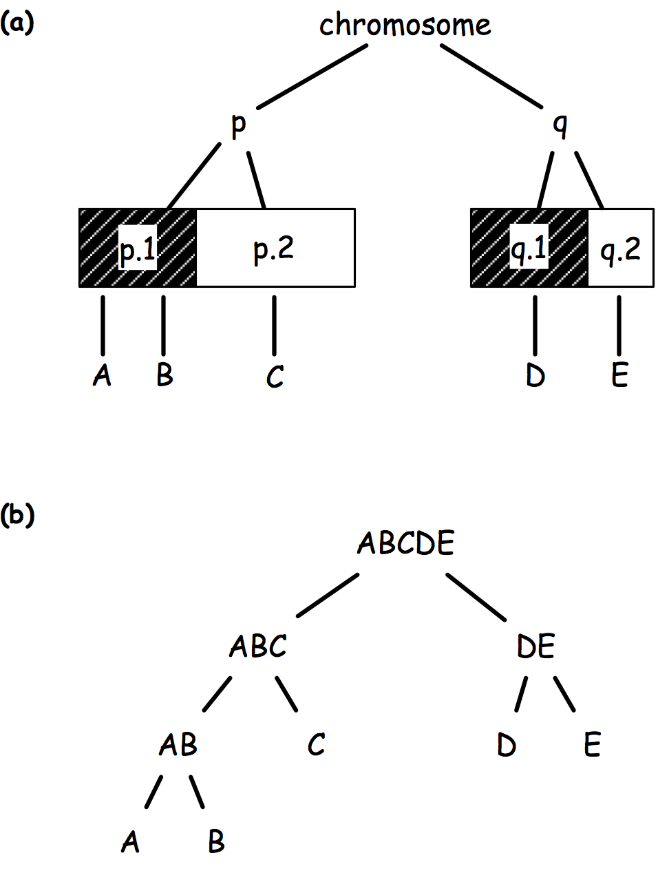
The sequential rejection principle states that if one hypothesis is rejected, then we might update the remaining ones and set a new critical level for un-rejected hypothesis. Goeman and Solari⁽¹⁾ use this method throughout their inheritance procedure, but basically it derives from Meinshausen’s procedure:⁽²⁾ if hypothesis are arranged in a tree, critical levels are found to be equal to alpha * # letters / # leaves. Figure 2 shows an example of how hypotheses and critical levels are processed.

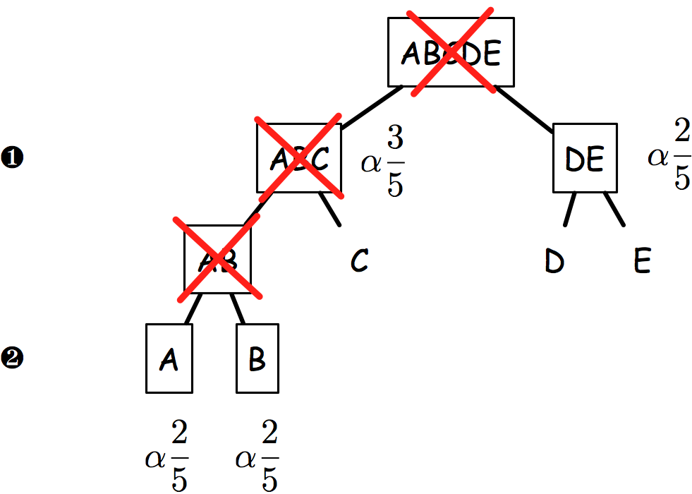
In the latest case (on the right), if AB is rejected, then it follows that both A and B critical levels are alpha x 2/5 since if AB is false, we know that at least one of A or B is false.

The authors then illustrate their testing procedure using a small data set of SNPs, but basically it is what is implemented in the globaltest R package. So, in what follows, I just try to mimic their example from the on-line help. It is to be noted that a permutation test is used to assess if the incorporation of structure information increases statistical power. I wonder how such resampling procedure might be tuned to handle large (real) data sets with 1M SNPs.

library(globaltest)
data(vandeVijver)
data(annotation.vandeVijver)
gt <- globaltest(vandeVijver, "StGallen", annotation.vandeVijver)
sampleplot(gt[1])
sp <- sampleplot(gt[1], plot = FALSE)
plot(sort(sp))

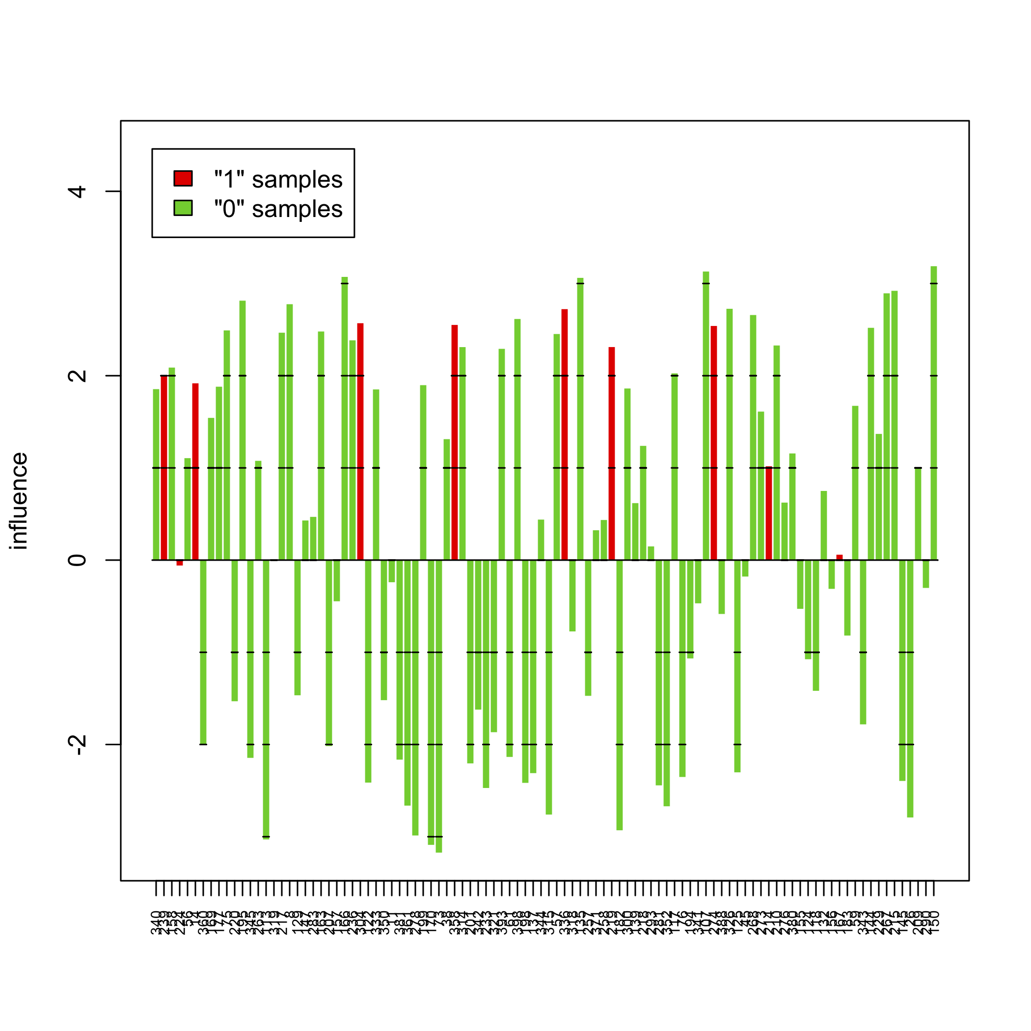
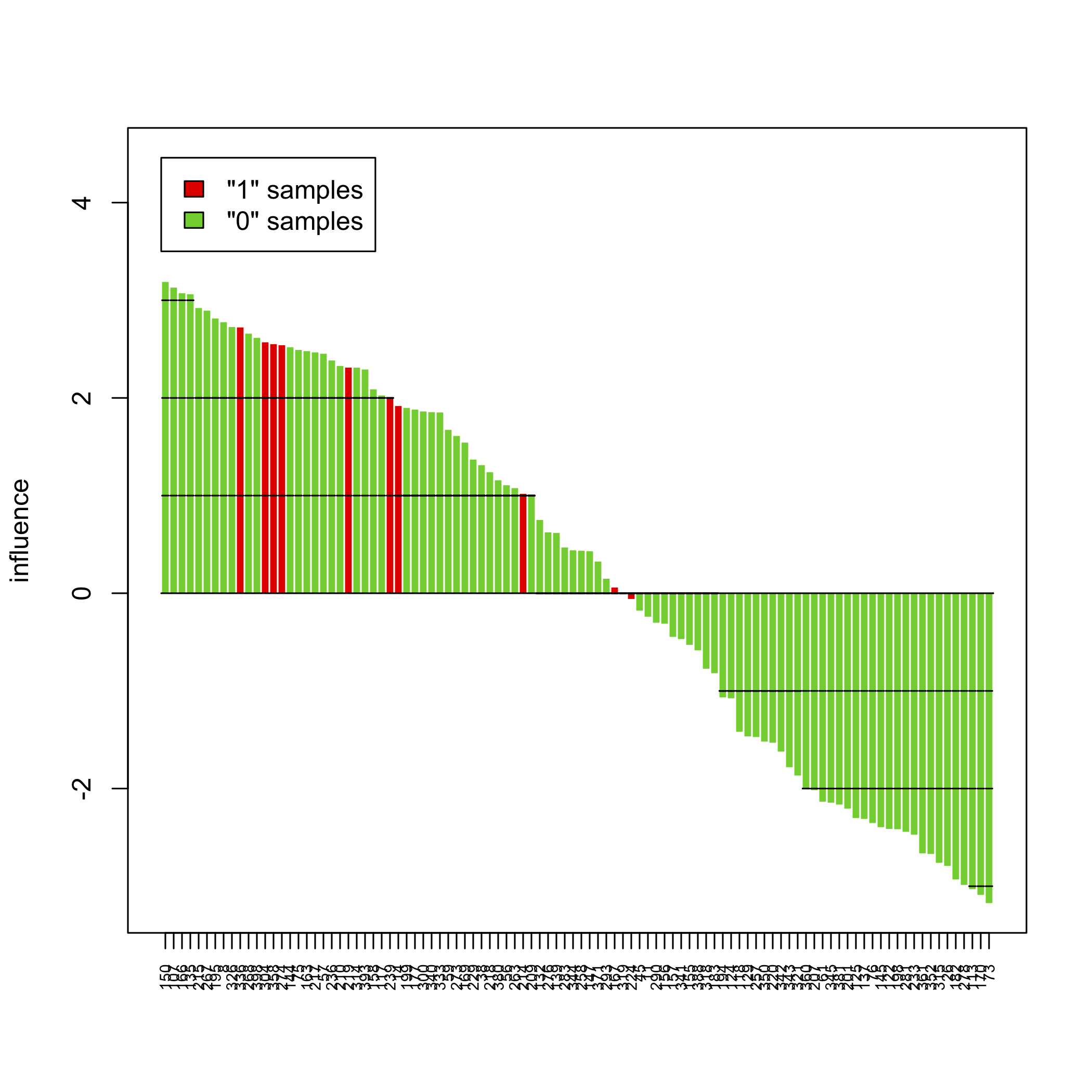
The above pictures show the influence of individual samples on the test result, but see the accompanying vignette (PDF) for more information.

Bayesian adjustment for multiplicity (J. Berger)

He gave a nice talk about problem frequently encountered in the USA with the results reproducibility. As an example, he provides the following numbers for clinical trials:

• during phase I, there are 8% of chance for reaching market, whereas it was 14% 15 years ago;
• there is actually a 70% of failure rates in phase III, whereas it was 20% 10 years ago;
• reports where 30% of phase III successes are observed actually failed to replicate.

This motivating illustrations should alert the reader that too many RCTs failed to reach a satisfactory level of evidence, and this may largely due to problem with multiple comparisons. Bayesian analysis deals with adjustment for multiplicity of testing solely through the assignment of prior probabilities to models or hypotheses.

If we note $X_i \sim N(\mu; 1)$, $i = 1, \dots, m$, a set of predictors, whose correlation is $\rho$, then two cases can be distinguished based on the value of $\rho$:

• if $\rho = 0$ (independent case), then we can set the critical level at $\alpha / m$ (Bonferonni method);
• if $\rho > 0$, it can be shown that

$$ \alpha = \Pr(\max_i X_i > K \mid \mu_1 = \dots = \mu_m = 0) = \mathbb E^Z\left[1-\Phi\left( \frac{K - \sqrt{\rho}Z}{\sqrt{1 - \rho}}\right)^m\right], $$

where $Z$ and $\Phi$ refer to the standard normal density and CDF. When $\rho = 0$, it approximates the Bonferonni solution, and

$$ \alpha\underset{p\to 1}\rightarrow 1-\Phi(K). $$

It may also be worth looking at Bayesian Model Averaging.

A couple of references about non-mutually exclusive bayesian multiple testing:

1. Scott, J.G. and Berger, J.O. (2006). Bayes and empirical-Bayes multiplicity adjustment in the variable-selection problem. Ann. Statist. 38(5): 2587-2619.
2. Gönen, M., Westfall, P.H., and Johnson, W.O. (2003). Bayesian Multiple Testing for Two-Sample Multivariate Endpoints. Biometrics 59(1): 76-82.
3. Müller, P., Parmigiani, G., and Rice, K. (2006). FDR and Bayesian Multiple Comparisons Rules. Proc. Valencia / ISBA 8th World Meeting on Bayesian Statistics Benidorm (Alicante, Spain), June 1st–6th.
4. Storey, J.D., Dai, J.Y., and Leek, J.T. (2007). The optimal discovery procedure for large-scale significance testing, with applications to comparative microarray experiments. Biostatistics 8: 414-432.

Local sparse bump hunting for finding groups in high-dimensional data (J.-E. Dazard)

This talk focused on semi-supervised methods seeking local patterns in data, for cluster analysis or classification. The “bump hunting” framework allows to find regions in the feature space with relatively high or low values for the target variable, see e.g., Bump Hunting in High-Dimensional Data, from Friedman and Fisher. The original work is described here: Friedman, J.H. and Fisher, N.I. (1999). Bump-hunting for high dimensional data. *Statistics and Computing 9: 123-143.

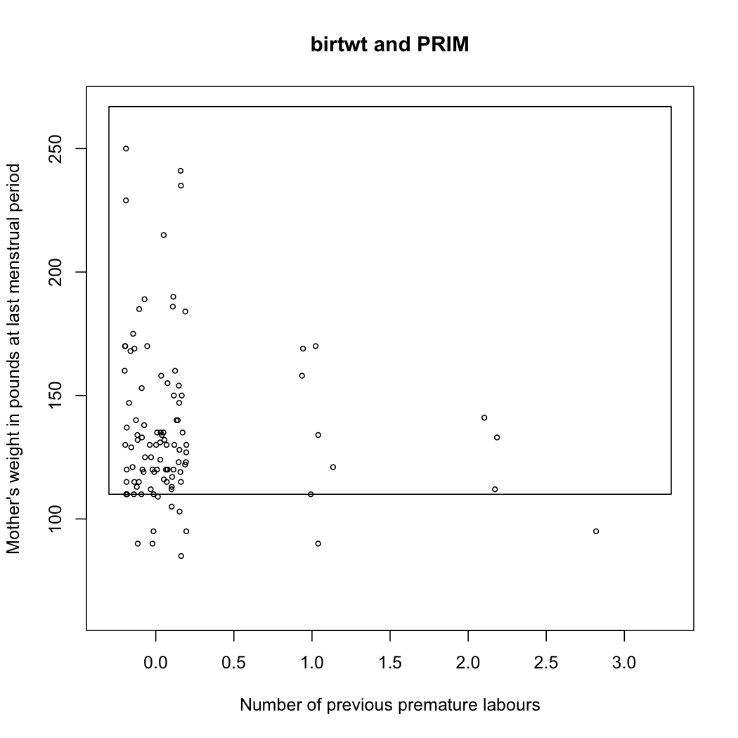
The prim package follows from this seminal work and allows to fit PRIM models (See its accompanying vignettes, e.g., Using prim for bump hunting). For instance, let’s consider the birthwt data, which comes from a study on risk factors associated with low infant birth weight.

data(birthwt, package="MASS")
x <- with(birthwt, 
          data.frame(as.logical(smoke),as.logical(ht),ptl,lwt))
y <- birthwt$bwt
summary(birthwt.prim <- prim.box(x=x[,3:4], y=y, threshold.type=1))
plot(birthwt.prim, col="transparent",
     xlab="Number of previous premature labours",
     ylab="Mother's weight in pounds at last menstrual period")
points(jitter(x[y>2900,3]),x[y>2900,4], cex=.6)

Here is the resulting bounding box found by the PRIM algorithm:

Turning back to the talk, the author presents an algorithm for Local Sparse Bump Hunting (LSBH) which I roughly summarize as: (1) use CART for partitioning the input space, (2) use (local) sPCA followed by a rotation, and a test for identifying local, which, if positive, is followed by PRIM, (3) aggregation of the results. This does not make any MVN assumption. In short, LSBH is a combination of greedy and patient methods, going recursively and locally. It should be available as an R package (lshb).

Identifying SNP interactions by cluster-localized sparse logistic regression (H. Binder)

The author is interested in studying main and epistatic effects in genomic studies, especially SNPs data. Here, the data set under consideration was composed of 312,624 SNPs genotyped on N=1272 patients (336 cases, 936 controls) in a clinical trial on urinary bladder cancer.

Harald Binder has already made great work in the domain of boosting regression and localized classification, especially:

1. Tutz, G. and Binder, H. (2007). Boosting ridge regression. Computational Statistics & Data Analysis 51: 6044-6059.
2. Tutz, G. and Binder, H. (2005). Localized classification. Statistics and Computing 15: 155-166.

He also worked on GAMs and a nice review is available online: Fitting Generalized Additive Models: A Comparison of Methods. He also authored the GAMBoost package.

Here the talk deals with sparse regression modeling where we first make use of a clustering approach to identify covariates locally unimportant for prediction, then we fit a final local model. In short, it relies on a sparse fit by component-wise likelihood-based boosting, where the number of boosting steps is chosen by 10-fold CV. This extends the work from Friedman and Meulman (2004) who presented a distance-based algorithm to cluster attribute value data (JRSS B 66(4): 815-849). A preprint of this article is available here (PDF).

The R package SNPLClust should implement this statistical framework soon.

Detection of epistatic interactions in schizophrenic children (I. Ruczinski)

The slides are available on Ruczinski’s website, http://biostat.jhsph.edu/~iruczins.

Ingo Ruczinski has made great effort for developing the use of logic regression in epidemiological studies, with a particular emphasis on SNP data. Among the R packages he authored, there are:

• LogicReg, the base package for doing logic regression
• trio, for the detection of disease-associated SNP interactions in case-parent trio data
• logicFS, for the identification of SNP-SNP interactions

Estimating the number of true discoveries in a genome-wide association study (Y. Pawitan)

Although schizophrenia is a highly heritable disease (60-70% of heritability), there are still no known major genes. The author describes a case-control study (N=6909, fine mapping) based on the International Schizophrenia Consortium, which originally included 780k SNPs subsequently pruned to a set of almost independent 74,062 SNPs (based on LD).

The problem with GWAS is that we expect very few true associations, so most significant results are false positives. The FDR is usually about 100%, so it is not an interesting measure. The idea is rather to estimate the number of true discoveries $S(c) = R(c)-mc$, where $m$ is the number of SNPs, and $R(c)$ is the number of SNPs where $p < c$. In this case, $mc$ is approximately the number of top SNPs. The question then arises as to how we get a confidence band for $S(c)$. Using a permutation test (based on case/control labels) yields a p-value, but not CIs. However, CIs can be derived from the percentile of $S^\star(c)$, if we assume a logical requirement of monotonicity. But, it generates a substantial bias (of the same order as the signal if the signal is small), given that

$$ \mathbb E S(c)=m^{\frac{1}{2}}\mathbb E \big(\sup_{x<c}B(x)\big)\approx 0.798(mc)^{\frac{1}{2}} $$

For example, with $mc = 400$ top SNPs, the bias would be about 16.

I cannot remember why I noted the following reference, but the number of subjects (>100,000) used to highlight novel loci associated to plasma lipids looks impressive: Teslovich, T.M., Musunuru, K., Smith, A.V., et al. (2010). Biological, clinical and population relevance of 95 loci for blood lipids (PDF), *Nature 466: 707-713.

A marginal global two-sample test for multivariate (high-dimensional) binary data (U. Mansmann)

The author used ICF to select data from stroke patients (ICF includes about 1662 items arranged in a hierarchical structure) and applied GEE on the resulting binary outcomes. The aim of this talk was on multiple testing strategies to focus global testing.

Basically, he derived a statistic looking like $\sum_{i=1}^pT_i = U^tWU$.

with $T_i$ distributed as a $\chi^2$ at every single item (crossed by gender). The idea was then to replace the component-wise $\chi^2$ by a component-wise logistic regression, and to apply an LR test on model with and without the interaction term.

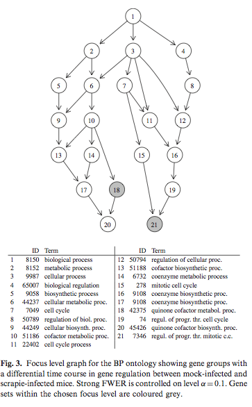
Simulated correlated multivariate binary data were generated with the bindata package. Hierarchical testing of variable importance follows the Meinshausen’s method, already discussed at the top of this page. The following picture is taken from Hummel et al.⁽¹⁾ and it shows results from the focus level procedure that determined a subgraph of the GO with a controlled number of falsely rejected null hypotheses.

Interesting references to work throughout are:

1. Hummel, M., Meister, R., and Mansmann, U. (2007). GlobalANCOVA: exploration and assessment of gene group effects. Bioinformatics 24(1): 78-85.
2. Bousquet, C., Henegar, C., Louët, A.L., Degoulet, P., and Jaulent, M.C. (2005). Implementation of automated signal generation in pharmacovigilance using a knowledge-based approach. Int J Med Inform 74(7-8): 563-571.

Bootstrapped power enhanced multiple testing (R. Mukherjee)

This talk was about the problem of size allocation, that is how to setup individual type I error rate to control FWER or FDR. Bonferroni and Sidak’s methods rely on equally sized tests. Papers from Spjøtvoll⁽¹⁾ and Storey⁽²⁾ discuss how to control the expected number of false rejections. In another paper, Pena et al.⁽³⁾ described the missed discovery rate (MDR) and showed that minimizing MDR is equivalent to maximizing the average power.

1. Spjøtvoll, E. (1972). On the Optimality of Some Multiple Comparison Procedures. The Annals of Mathematical Statistics 43: 398-411.
2. Storey, J.D. (2007). The optimal discovery procedure: a new approach to simultaneous significance testing. JRSS B 69(3): 347-368.
3. Pena, E.A., Habiger, J. and Wu, W. (2010). Power-Enhanced Multiple Decision Functions Controlling Family-Wise Error and False Discovery Rates. Submitted to Ann. Statist, available on arXiv 0908.1767.

Discovering gene networks using L1 and L0 penalties (J. de Rooi)

Considering the huge amount coming from gene expression studies, the natural question that comes to mind is: What does the dependency structure among the genes look like?

One way to answer this question is to use Graphical Models. A good starting point on GGM is Introduction to Graphical Modelling, from D. Edwards (Springer, 2000) or the ggm package. They have been successfully used by Krämer et al.⁽¹⁾, who also authored the parcor package. Several approaches were already described, including (1) topology models, (2) control logic models, or (3) dynamic models. The authors focused on the first approach which aims to identify modules and hubs in the underlying graph. Modules allow to model the strongest dependencies among the genes and to obtain a sparse representation in turn.

When $p > n$, the covariance matrix is ill-conditioned or singular, so it calls for penalized regression. Basically, we fit p regression models and look at the partial correlation coefficient defined as

$$ \rho_{ij\cdot z}=\text{sign}(\beta_{ij})\sqrt{\beta_{ij}\beta_{ji}} $$

which is $\neq 0$ iff $\text{sign}(\beta_{ij})=\text{sign}(\beta_{ji})$. This is a smooth approximation to the L0 penalty. So, we start fitting a model with L1 penalty, then we use its final estimates as starting points for L0 penalization. The whole procedure is encompassed within a cross-validation procedure. Results on simulated random or structured networks are compared to existing methods such as PLS,⁽²⁾ L1 regression,⁽³⁾ adjusted-L1 regression,⁽⁴⁾ and PCIT.⁽⁵⁾

Overall, the results showed that PLS and PCIT generate many false positives, and that both aL1 and L0 returned the highest precision. L0 tend to create large bias in terms of MSE. In conclusion, the aL1 method seems to be the best method.

1. N. Kraemer, J. Schaefer, A.-L. Boulesteix (2009). Regularized estimation of large-scale gene regulatory networks using Gaussian Graphical Models. BMC Bioinformatics 10: 384.
2. cannot remember the reference :(
3. Rothman, A., Levina, L., and Zhu, J. (2009). Generalized thresholding of large covariance matrices. JASA 104: 177-186.
4. Zou, H. (2006). The adaptive Lasso and its oracle property. JASA 101(476): 1418-1429.
5. Reverter, A. and Chan, E.K.F. (2008). Combining partial correlation and an information theory approach to the reversed engineering of gene co-expression networks. Bioinformatics 24(21): 2491-2497. See the PCIT package.