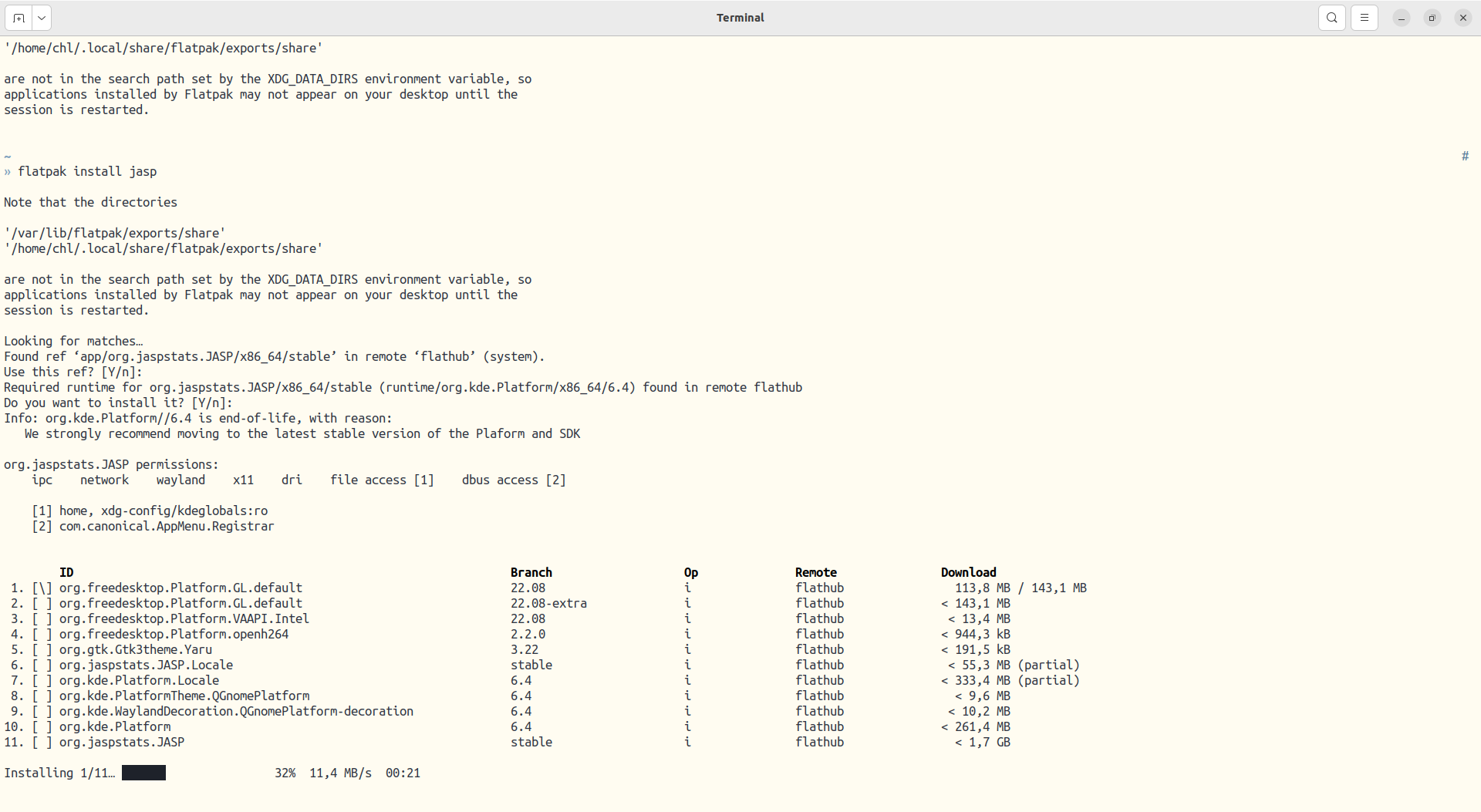
I installed JASP recently as I wanted to see how it evolves since the last time I used it (several years ago). Unfortunately, there’s no package, tarball or AppImage so you need to install it from Flathub, using flatpak. With regard to my last post, this also was an occasion to try out flatpak. Overall, it works quite well, it doesn’t update itself or its packages de manière impromptue, and it is simple to use. Of course, you end up with giant applications since it bundles every dependencies it needs. For instance, JASP is as large as 2.6 Go once installed in /var/lib/flatpak. Anyway, the installation went smoothly, and I came to appreciate the flatpak way of installing desktop app. I might even replace all my AppImage’s with those from Flathub.¹

Back to Bayesian statistics. Several years ago I mentioned a Bayesian alternative to the traditional Student t-test, but the post found its way into the draft folder forever. Rather than writing and submitting to Stan or JAGS a model file, here is what I would do in R. First, using the brms package, we can mimic a t-test assuming unequal variance as follows:

> library(brms)
> m <- brm(bf(len ~ supp, sigma ~ supp), data = ToothGrowth, family = student, cores = 4)
--8<------ snip --
> summary(m)
 Family: student
  Links: mu = identity; sigma = log; nu = identity
Formula: len ~ supp
         sigma ~ supp
   Data: ToothGrowth (Number of observations: 60)
  Draws: 4 chains, each with iter = 2000; warmup = 1000; thin = 1;
         total post-warmup draws = 4000

Population-Level Effects:
                Estimate Est.Error l-95% CI u-95% CI Rhat Bulk_ESS Tail_ESS
Intercept          20.89      1.27    18.41    23.45 1.00     5225     2737
sigma_Intercept     1.87      0.14     1.59     2.15 1.00     4015     2762
suppVC             -4.01      2.00    -7.84    -0.13 1.00     4398     2992
sigma_suppVC        0.22      0.20    -0.16     0.61 1.00     4197     2944

Family Specific Parameters:
   Estimate Est.Error l-95% CI u-95% CI Rhat Bulk_ESS Tail_ESS
nu    25.77     14.91     6.55    62.61 1.00     4616     2776

Draws were sampled using sampling(NUTS). For each parameter, Bulk_ESS
and Tail_ESS are effective sample size measures, and Rhat is the potential
scale reduction factor on split chains (at convergence, Rhat = 1).
>

The tidybayes package is a handy companion if you work with brms objetcs. We can compare the above results with what would be obtained from the now archived BEST package (latest version is from 2021):²

> library(BEST)
> grp <- with(ToothGrowth, split(len, supp))
> BESTmcmc(grp[[1]], grp[[2]], parallel = TRUE)
Waiting for parallel processing to complete...done.
MCMC fit results for BEST analysis:
100002 simulations saved.
         mean      sd median  HDIlo   HDIup Rhat n.eff
mu1    20.797  1.2951 20.798 18.254  23.372    1 61131
mu2    16.889  1.6041 16.890 13.796  20.098    1 62000
nu     42.396 31.2307 34.208  3.113 104.074    1 24364
sigma1  6.765  0.9835  6.666  4.953   8.723    1 47897
sigma2  8.449  1.2427  8.314  6.178  10.928    1 43607

'HDIlo' and 'HDIup' are the limits of a 95% HDI credible interval.
'Rhat' is the potential scale reduction factor (at convergence, Rhat=1).
'n.eff' is a crude measure of effective sample size.

This takes a much shorter amount of time. Kruschke wrote a paper about this approach, ³ which is implemented by the above function call. From the on-line help:

The function uses a t-distribution to model each sample, and generates vectors of random draws from the posterior distribution of the center (mu) and spread or scale (sigma) of the distribution, as well as a measure of normality (nu). The procedure uses a Bayesian MCMC process implemented in JAGS ⁴.

Kruschke also discussed two-group comparisons in section 16.3 of the second edition of his famous textbook.⁵ As noted by the author, “When using t distributions for robust estimation, we could also estimate the normality of each group separately. But because there usually are relatively few outliers, we will use a single normality parameter to describe both groups, so that the estimate of the normality is more stably estimated.”

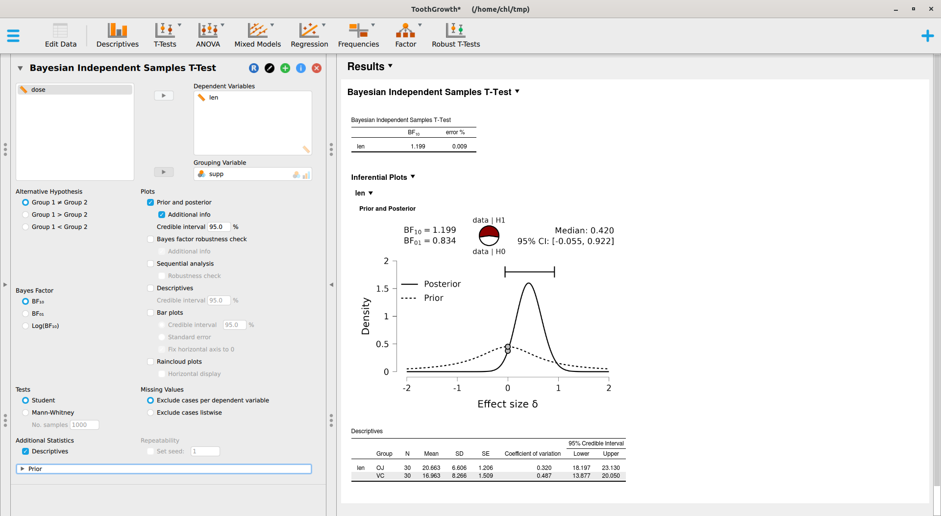
Now, it’s time to try out JASP. Here’s what we get after specifying an informed prior (Student t distribution with default scale factor of 0.707 and df=1) instead of a scaled Cauchy distribution:

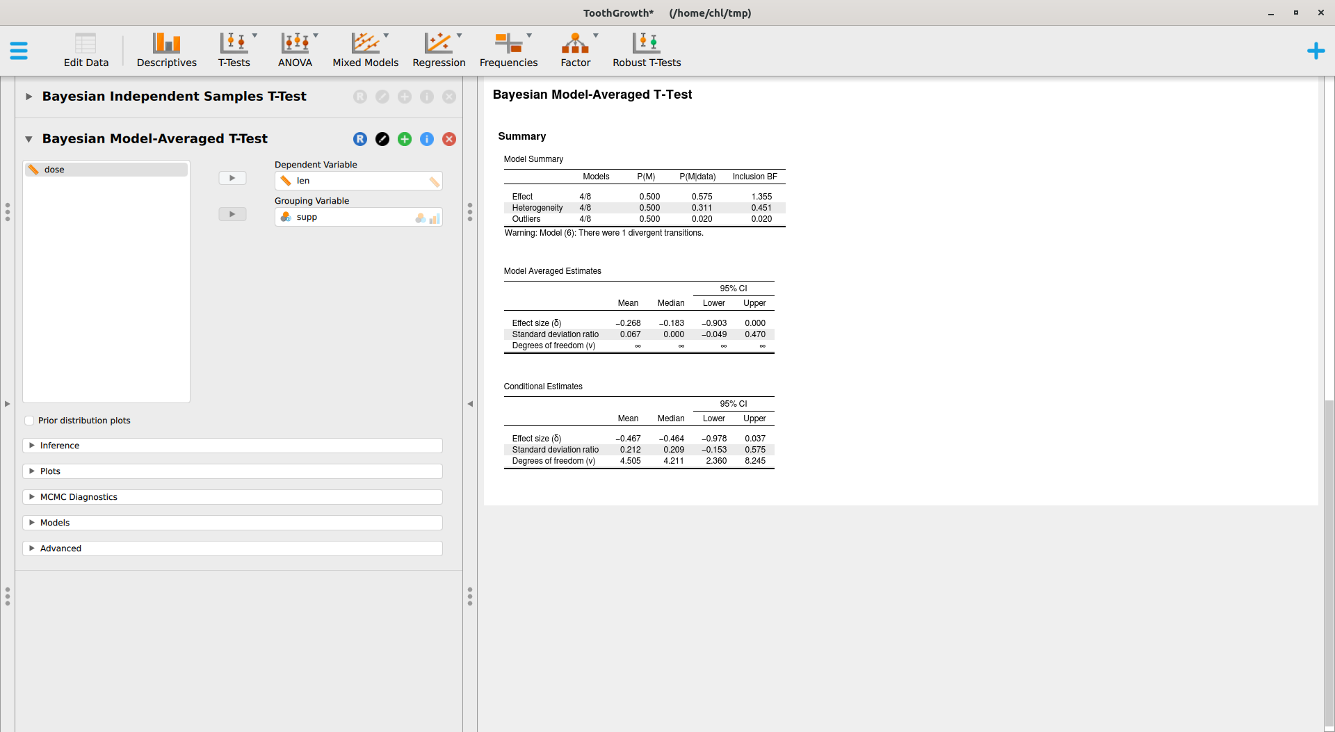
This module relies on the BayesFactor package, where the ttestBF implements work made by Morey and coll.⁶ JASP also offers a Robust T-Tests module which provides Bayesian model-averaged t-test, as implemented in the RoBTT package. See also A conceptual introduction to Bayesian Model Averaging for an introduction. This involves longer computation time, but with default parameters we obtain the following results:

There are various options that I did not try, but overall I find that this is a great way to get started with Bayesian statistics for beginner students. No need to learn complex R code or to install various stuff. However, we need to carefully check what packages are used under the hood, what priors are used, and what statistics are reported (e.g., Bayes Factor, posterior estimates, etc.).