lost+found 2014
Here are some draft notes, written in 2014, unfilled but not lost forever. With slight edits to accommodate a proper archive blog post.
Stata for structural equation modeling
(October 2014)
As Mplus syntax often appears a bit cryptic to carry out basic operations in Confirmatory Factor Analysis (CFA), I decided to write out some of the notes I took when using Mplus for recent psychometric studies.
In what follows, I will use data described and analyzed in Acock’s Stata textbook, Discovering Structural Equation Modeling Using Stata. Why this book? Essentially because it provides a ready-to-use dataset [describe it here], and the author discusses several applications of CFA models, including tests for measurement invariance, without much technical details. For those interested in a more rigorous approach, I can recommend Structural Equation Modeling. Applications Using Mplus, by Wang & Wang (2012, Wiley).
Multigroup analysis
In this post, I am interested in assessing weak and strong measurement invariance using Stata and Mplus. Both are popular statistical packages, and although these are commercial software they are worth their price, IMHO. Mplus includes more estimators than Stata, but probably we could tweak Stata commands to mimic Mplus.
A tutorial on multi-group CFAs with Stata can be found on the UCLA server: How can I check measurement invariance using the sem command?. Basically, measurement invariance can be assessed by fitting several nested models, where we impose additional constraints at each stage:
- (M1) all parameters free
- (M2) metric (pattern) invariance – loadings are invariant
- (M3) strong (scalar) invariance – loadings & intercepts are invariant
- (M4) strict invariance – loadings, intercepts & residuals are invariant
- (M5) strict invariance plus factor means are invariant
- (M6) strict invariance plus factor means & variances are invariant
Configural invariance is usually assessed using M1, the idea being to check that the hypothesized factor structure holds in all groups. It is also used as a reference (or baseline) model against which other models will be tested. Model M2 is the first step to demonstrate weak measurement invariance, that is M1 holds (i.e., factor loadings are as expected in all groups) but in addition loadings are equal in all subpopulations. We only allow item intercepts to differ between subgroups. Model M3 is used to test strong measurement invariance where in addition to loadings we impose that item intercepts are equal in all groups. A more constrained model, M4, also adds the constraint of equal errors of measurement. This model, and models M5-M6 are generally too strong, and hard to verify; after all, we only have one sample, and many researchers would be quite happy with demonstrating that strong measurement invariance is verified. [add reference]
To get the dataset under Stata, we write:
. use http://www.stata-press.com/data/dsemus/multgrp_cfa.dta
To create a standalone text file we will use the handy Stata program Stata2mplus, which allows to convert Stata data file to Mplus input file. This is easier than using Stata built-in converters since it will recode missing values, remove header, and select the correct field delimiter:
. stata2mplus using multgrp_cfa
This generates two files:
$ ls multgrp_cfa.*
multgrp_cfa.dat  multgrp_cfa.inp
where the Mplus file contains details about items that were converted and basic syntax to read the dat file later:
Data:
  File is multgrp_cfa.dat ;
Variable:
  Names are
     female x1 x2 x3 x4 x5 x6 x7 x8 x9 x10 x11 x12 x13;
  Missing are all (-9999) ;
Analysis:
  Type = basic ;
The sample is composed of 8,984 respondents, with about 50% of men and women.
. tabulate female

     female |      Freq.     Percent        Cum.
------------|-----------------------------------
        Man |      4,599       51.19       51.19
      Woman |      4,385       48.81      100.00
------------|-----------------------------------
      Total |      8,984      100.00
Basic item statistics are provided below, as mean ± SD and range, and values for Cronbach alpha (unstandardized since all responses are expressed on the same 4-point scale):
. summarize x1-x3 x4 x9 x10 x12

    Variable |       Obs        Mean    Std. Dev.       Min        Max
-------------|--------------------------------------------------------
          x1 |      7351     3.24092    .6674483          1          4
          x2 |      7474    2.188788    .6645846          1          4
          x3 |      7375    3.659119    .5932246          1          4
          x4 |      1833    2.331697    1.022223          1          4
          x9 |      1811    2.276643    .9320571          1          4
-------------|--------------------------------------------------------
         x10 |      1775    2.228732    1.072652          1          4
         x12 |      1847    1.705468    .7425231          1          4


. alpha x1-x3 x4 x9 x10 x12, item

Test scale = mean(unstandardized items)

                                                            average
                             item-test     item-rest       interitem
Item         |  Obs  Sign   correlation   correlation     covariance      alpha
-------------|-----------------------------------------------------------------
x1           | 7351    +       0.6973        0.3609        .1536247      0.6926
x2           | 7474    -       0.5810        0.3359        .1781062      0.7343
x3           | 7375    +       0.6428        0.3033        .1663125      0.6999
x4           | 1833    +       0.6226        0.3684        .1494082      0.7191
x9           | 1811    +       0.6401        0.4216         .147084      0.7077
x10          | 1775    +       0.6541        0.3978        .1432081      0.7101
x12          | 1847    +       0.6349        0.4660        .1504138      0.7027
-------------|-----------------------------------------------------------------
Test scale   |                                             .1541296      0.7398
-------------------------------------------------------------------------------
As can be seen, there are many missing data for items x4, x9, x10, and x12, which means that the sample size will be considerably reduced when using available data.
Fitting a baseline model
A model imposing equivalent form on all relationships between items and factors in men and women, but no equality constraints, can be fitted as follows:
. sem (Depress -> x1 x2 x3) (Gov_Resp -> x4 x9 x10 x12), group(female) ginvariant(none) means(Depress@0 Gov_Resp@0)
(7377 observations with missing values excluded)

Endogenous variables

Measurement:  x1 x2 x3 x4 x9 x10 x12

Exogenous variables

Latent:       Depress Gov_Resp

Fitting target model:

Iteration 0:   log likelihood = -12363.307
Iteration 1:   log likelihood = -12362.434
Iteration 2:   log likelihood =  -12362.43
Iteration 3:   log likelihood =  -12362.43

Structural equation model                       Number of obs      =      1607
Grouping variable  = female                     Number of groups   =         2
Estimation method  = ml
Log likelihood     =  -12362.43

 ( 1)  [x1]0bn.female#c.Depress = 1
 ( 2)  [x4]0bn.female#c.Gov_Resp = 1
 ( 3)  [mean(Depress)]0bn.female = 0
 ( 4)  [mean(Gov_Resp)]0bn.female = 0
 ( 5)  [x1]1.female#c.Depress = 1
 ( 6)  [x4]1.female#c.Gov_Resp = 1
 ( 7)  [mean(Depress)]1.female = 0
 ( 8)  [mean(Gov_Resp)]1.female = 0

---%<-------------------------------------------------------------------------

LR test of model vs. saturated: chi2(26)  =     51.00, Prob > chi2 = 0.0024

. estat gof, stats(all)

----------------------------------------------------------------------------
Fit statistic        |      Value   Description
---------------------|------------------------------------------------------
Likelihood ratio     |
         chi2_ms(26) |     50.999   model vs. saturated
            p > chi2 |      0.002
         chi2_bs(42) |   2312.800   baseline vs. saturated
            p > chi2 |      0.000
---------------------|------------------------------------------------------
Population error     |
               RMSEA |      0.035   Root mean squared error of approximation
 90% CI, lower bound |      0.020
         upper bound |      0.049
---------------------|------------------------------------------------------
Information criteria |
                 AIC |  24812.859   Akaike's information criterion
                 BIC |  25049.673   Bayesian information criterion
---------------------|------------------------------------------------------
Baseline comparison  |
                 CFI |      0.989   Comparative fit index
                 TLI |      0.982   Tucker-Lewis index
---------------------|------------------------------------------------------
Size of residuals    |
                SRMR |      0.030   Standardized root mean squared residual
                  CD |      0.945   Coefficient of determination
----------------------------------------------------------------------------
Note: pclose is not reported because of multiple groups.
The key options are group(female) ginvariant(none), which indicate that we want to consider a grouping factor but we do not want to add constraints on the measurement model in each group. Factor means are constrained to equal 0 in both groups, but not their variances.
With Mplus, we would use the following script. Note that Mplus does not use listwise deletion by default, so we have to specify this ‘non-feature’ using listwise is on; in order to ensure we are working with the same set of 1,607 subjects. With Mplus, factor means are written as is while factor variances are put into brackets. Constraints are represented by the symbol @. So [DEP@0] means that variance for factor Depression is constrained to be zero. For multi-group analysis, we need to add a GROUPING = option, and this will be used to formulate different factor structure (or constraints) in each group, as indicated by each MODEL: step.
Data:
  File is multgrp_cfa.dat ;
LISTWISE is ON;
Variable:
  NAMES = female x1 x2 x3 x4 x5 x6 x7 x8 x9 x10 x11 x12 x13;
  USEVARIABLES = x1-x3  x4 x9 x10 x12;
  GROUPING = female (0=M 1=F);
  MISSING are ALL (-9999) ;
MODEL:
  DEP BY x1@1 x2-x3*;
  GOV BY x4@1 x9* x10* x12*;
  DEP*; GOV*;     ! free factor variances
  [DEP@0 GOV@0];  ! zero factor means
MODEL F:
  DEP BY x1@1 x2-x3*;
  GOV BY x4@1 x9* x10* x12*;
OUTPUT:
  TECH1 TECH4;
Results are provided below. Unless we specify the type of estimator we want to use, Mplus will default to an ML estimator, as Stata did.
MODEL FIT INFORMATION

Number of Free Parameters                       37

Loglikelihood

          H0 Value                      -12386.664
          H1 Value                      -12336.930

Information Criteria

          Akaike (AIC)                   24847.328
          Bayesian (BIC)                 25046.467
          Sample-Size Adjusted BIC       24928.925
            (n* = (n + 2) / 24)

Chi-Square Test of Model Fit

          Value                             99.468
          Degrees of Freedom                    33
          P-Value                           0.0000

Chi-Square Contribution From Each Group

          M                                 44.009
          F                                 55.459

RMSEA (Root Mean Square Error Of Approximation)

          Estimate                           0.050
          90 Percent C.I.                    0.039  0.062
          Probability RMSEA <= .05           0.476

CFI/TLI

          CFI                                0.971
          TLI                                0.963

Chi-Square Test of Model Fit for the Baseline Model

          Value                           2312.800
          Degrees of Freedom                    42
          P-Value                           0.0000

SRMR (Standardized Root Mean Square Residual)

          Value                              0.049
The chi-square test that is reported under the term ‘baseline vs. saturated’ (Χ2(42) = 2312.800, p < 0.001) corresponds to what Mplus call ‘Chi-Square Test of Model Fit for the Baseline Model’, whereas that headed ‘model vs. saturated’ (Χ2(26) = 50.999, p = 0.002) is called ‘Chi-Square Test of Model Fit’ in Mplus.
FIXME: explain why DF differ between the two software!
Testing for invariance of factor loadings
With Stata, we just add ginvariant(mcoef) to constrain factor loadings to be equal in both groups. Using Mplus, we will just remove everything under the MODEL F: part, meaning that factor loadings for women will no longer be estimated freely but constrained to be qual to those of men.
Here are Mplus results:
MODEL FIT INFORMATION

Number of Free Parameters                       32

Loglikelihood

          H0 Value                      -12389.320
          H1 Value                      -12336.930

Information Criteria

          Akaike (AIC)                   24842.639
          Bayesian (BIC)                 25014.867
          Sample-Size Adjusted BIC       24913.209
            (n* = (n + 2) / 24)

Chi-Square Test of Model Fit

          Value                            104.779
          Degrees of Freedom                    38
          P-Value                           0.0000

Chi-Square Contribution From Each Group

          M                                 46.335
          F                                 58.444

RMSEA (Root Mean Square Error Of Approximation)

          Estimate                           0.047
          90 Percent C.I.                    0.036  0.058
          Probability RMSEA <= .05           0.675

CFI/TLI

          CFI                                0.971
          TLI                                0.967

Chi-Square Test of Model Fit for the Baseline Model

          Value                           2312.800
          Degrees of Freedom                    42
          P-Value                           0.0000

SRMR (Standardized Root Mean Square Residual)

          Value                              0.049
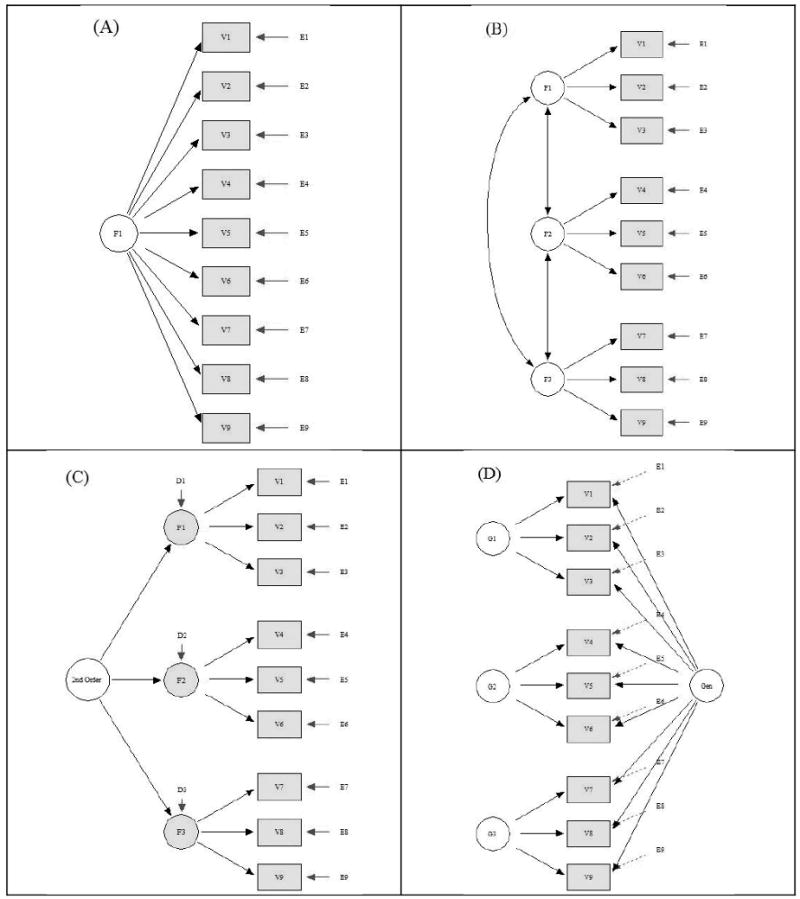
Bifactor models
Here are some notes on Bifactor models, and their use in psychological or medical research.
As illustrated in the following picture (taken from Reise et al., 2010; see full reference below), a bifactor model differs from a second-order factor model in that (1) factor (or primary units) are not correlated, (2) the relation between indicators or items and the general factor is direct, and not mediated by specific factors as in a second-order factor model. As such, the bifactor model may be seen as a measurement model, unlike the later.
From Statalist, I found the following references on second-order factor and bifactor models (whenever possible I fixed dead links and tried to find ungated PDFs):
- Koufteros, X., Babbarb, S., & Kaighobadi, M. (2009). A paradigm for examining second-order factor models employing structural equation modeling. International Journal of Production Economics, 120(2), 633-652.
- Rindskopf, D., & Rose, T. (1988). Some theory and applications of confirmatory second-order factor analysis. Multivariate Behavioral Research, 23(1), 51-67.
- Chen, F.F., West, S.G., & Sousa, K.H. (2006). A Comparison of Bifactor and Second-Order Models of Quality of Life. Multivariate Behavioral Research, 41(2), 189–225.
- Chen, F.F., Hayes, A., Carver, C.S., Laurenceau, J.-P., Zhang, Z. (2012). Modeling General and Specific Variance in Multifaceted Constructs: A Comparison of the Bifactor Model to Other Approaches. Journal of Personality, 80(1), 219-251.
- Landsheer, J.A. (2010). The specification of causal models with Tetrad IV: a review. Structural Equation Modeling, 17(4), 703-711.
- Zheng, Z.E., & Pavlou, P.A. (2010). Toward a Causal Interpretation from Observational Data: A New Bayesian Networks Method for Structural Models with Latent Variables. Information Systems Research, 21(2), 365-391.
- Xu, L. (2010). Machine learning problems from optimization perspective. Journal of Global Optimization, 47, 369–401.
- Tu, S., & Xu, L. (2011a). Parameterizations make different model selections: Empirical findings from factor analysis. Frontiers of Electrical and Electronic Engineering in China, 6(2), 256–274.
- Tu, S., & Xu, L. (2011b). An investigation of several typical model selection criteria for detecting the number of signals. Frontiers of Electrical and Electronic Engineering in China, 6(2), 245–255. http://www.cse.cuhk.edu.hk/~lxu/papers/journal/11FEE-tsk-sev.pdf ;
- Xu, L. (2011). Codimensional matrix pairing perspective of BYY harmony learning: hierarchy of bilinear systems, joint decomposition of data-covariance, and applications of network biology. Frontiers of Electrical and Electronic Engineering in China, 6(1), 86–119.
Here are some other references:
- Liu, T., Dai, H., and Zhao, Y. (2012). Comparison of Full-Information and Limited-Information Methods for Bi-Factor Model. Advances in information Sciences and Service Sciences (AISS), 4(11), 11-18.
- Chen, F.F., Sousa, K.H., and West, S.G. (2005). Testing Measurement Invariance of Second-Order Factor Models. Structural Equation Modeling, 12(3), 471-492.
- Resie, S.P, Moore, T.M., and Haviland, M.G. (2010). Bifactor Models and Rotations: Exploring the Extent to which Multidimensional Data Yield Univocal Scale Scores. Journal of Personality Assessement, 92(6), 544–559.
In an older post, I talked about formative vs. reflective measurement. Here are some slides that contain a lot more references.
Book review
Here are some notes on statistical books I read this (academic) year. This time, I will concentrate on psychometrics. Several books rely on Mplus.
-
Introduction to Psychometric Theory (Raykov & Marcoulides, 2011, Routledge). This is an interesting overview of ‘modern’ psychometrics, including factor analysis and item response theory. The authors provide a detailed account of reliability (chapters 6 and 7), and generalizability theory.
-
Data analysis with Mplus (Geiser, 2013, Guilford Press). This is a gentle introduction to the Mplus software for structural equation modeling (cross-sectional and longitudinal settings), latent class analysis and hierarchical multilevel models.
-
Discovering Structural Equation Modeling Using Stata (Acock, 2013, Stata Press). I really like books from Stata Press: they are generally well-written, background information is provided and applications are well targeted and illustrated. I already talked about this book as it was published along the new release of Stata 12 and its SEM builder. As always, additional material are available on the companion website.
-
Structural Equation Modeling. Applications Using Mplus (Wang & Wang, 2012, Wiley). This is a very nice book, with complete Mplus code to illustrate various models fitted on a short version of the Brief Symptoms Inventory (BSI-18).
-
Latent Variable Modeling Using R (Beaujean, 2014, Routledge)