lwb.R |
|
|---|---|
|
The low birth weight study (Hosmer and Lemeshow, 1989) will be
used to illustrate basic descriptive and inferential techniques in
R. This is a complete study, although analysis will somehow depart
from the one presented in Hosmer and Lemeshow’s textbook. |
|
Preparing the dataset |
|
Importing data |
|
|
The low birth weight dataset is already available in the |
library(MASS)
data(birthwt)
str(birthwt) |
|
To get a gentle numerical overview of the data, we can use the
|
summary(birthwt) |
|
The very first thing to do with unknown datasets is to check for the
presence of missing values (MV). This is done with |
apply(birthwt, 2, function(x) sum(is.na(x)))
dim(birthwt) |
Recoding and checking variables |
|
|
Some of the factors of interest will not be understood by R as we would
like it to do because they are just treated as numerical
variables. So, the next step is to convert them to (unordered)
|
birthwt <- within(birthwt, {
  low <- factor(low, labels=c("No","Yes"))
  race <- factor(race, labels=c("White","Black","Other"))
  smoke <- factor(smoke, labels=c("No","Yes"))
  ui <- factor(ui, labels=c("No","Yes"))
  ht <- factor(ht, labels=c("No","Yes"))
}) |
|
Again, with unknown data, it is recommended to take a close look at
the distribution of numerical variables, which in this particular
case can be isolated using a repeated call to |
idx <- sapply(birthwt, is.numeric) |
|
We then use box-and-whiskers charts to summarize each distribution. Note that we have rescaled them to avoid the problem of varying y-axis. |
boxplot(apply(birthwt[,idx], 2, scale)) |
Summarizing data |
|
|
Most base functions in R can be used to summarize our variables,
either numerically or graphically. We have already seen the useful
|
library(Hmisc)
summary(low ~ ., data=birthwt, method="reverse", overall=TRUE)
summary(bwt ~ ., data=birthwt)
summary(low ~ smoke + ht + ui, data=birthwt, fun=table) |
|
The above commands might be combined with the |
|
|
Multivariate displays can be used, essentially to study relationships between numerical variables or assess any systematic patterns of covariations. At this stage, it might be interesting to highlight individuals according to a certain characteristic (e.g., low birth weight). |
library(lattice)
parallel(birthwt[,idx], groups=birthwt$low, horizontal.axis=FALSE)
parallel(~ birthwt[,idx] | smoke, data=birthwt, groups=low,
         lty=1:2, col=c("gray80","gray20"))
splom(~ birthwt[,idx], data=birthwt, jitter.x=TRUE, cex=.6,
      groups=low, panel=panel.superpose, grid=TRUE,
axis.text.cex=0.6, xlab="", pch=c(2,6)) |
|
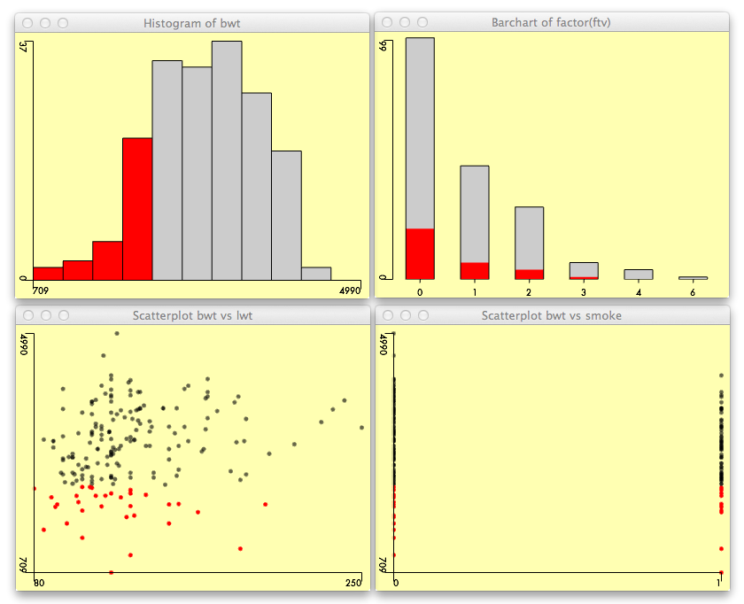
Visual exploration of the dataset can also rely on brushing and
linking techniques available in the ggobi
software, or directly with the
|
library(Acinonyx)
attach(birthwt)
iplot(lwt, bwt)
iplot(smoke, bwt)
ihist(bwt)
ibar(factor(ftv))
detach(birthwt) |
Dealing with continuous outcomes |
|
Assessing linear two-way relationships |
|
|
The covariation between mother’s weight in pounds at last menstrual period and birth weight can be assessed using a correlation test. Of course, we need to display the raw data in a scatterplot, first. It is possible to add a local regression line to the cloud of points to visually assess the linearity of the relationship. |
xyplot(bwt ~ lwt, data=birthwt, type=c("p", "smooth"))
with(birthwt, cor.test(bwt, lwt)) |
|
Compare the results to the ones obtained using Spearman’s method, which relies on ranks. |
with(birthwt, cor.test(bwt, lwt, method="spearman")) |
Comparing two means |
|
|
To test the hypothesis that there is no difference in baby weight depending on the smoking status (of the mother), we can use a t-test for independent samples where the standard error is computed from the pooled standard deviation (weighted average of sample SDs). |
t.test(bwt ~ smoke, data=birthwt, var.equal=TRUE) |
|
Omitting the |
t.test(bwt ~ smoke, data=birthwt) |
|
It is always a good idea to check whether the assumptions of the test are met, by computing the variances and displaying a quantile-quantile plot. This allows to judge the homogeneity of variances (but, don’t forget this is supposed to hold in the parent distributions) and the normality of the distributions. |
with(birthwt, tapply(bwt, smoke, var))
opar <- par(mfrow=c(1,2))
with(birthwt, qqplot(bwt[smoke=="No"], main=""))
with(birthwt, qqplot(bwt[smoke=="Yes"], main=""))
par(opar) |
|
In addition, we can produce a graphical summary of the two
distributions using boxplots or histograms. To superimpose a kernel
density estimate on the latter, see |
bwplot(bwt ~ smoke, data=birthwt)
histogram(~ bwt | smoke, data=birthwt, type="count") |
|
Should we want to use a non-parametric (distribution free)
statistic, we could apply a Wilcoxon test with |
|
Using re-randomization instead of parametric testing |
|
|
We could use a permutation technique instead of the t-test, and consider an approximate or exact distribution of the test statistic to decide whether there is a significant difference between central locations of the two groups. |
library(coin)
independence_test(bwt ~ smoke, data=birthwt, distribution="exact") |
Comparing more than two means |
|
|
In case we are interested in comparing more than two groups, we can use an ANOVA (instead of carrying out multiple unprotected t-tests). |
fm <- bwt ~ race
aov.fit <- aov(fm, data=birthwt)
summary(aov.fit) |
|
Again, it is good to check the distribution of the residuals. |
plot(aov.fit) |
|
The |
model.tables(aov.fit)
plot.design(fm, data=birthwt) |
|
Likewise, a two-way ANOVA can be used to test whether birth weight
depends on both smoking status and history of hypertension. If we
consider a saturated model, we need to include the interaction
|
summary(aov.fit2 <- aov(bwt ~ smoke * ht, data=birthwt))
with(birthwt, interaction.plot(smoke, ht, bwt)) |
|
As the interaction appears to be non significant, we can remove this term and fit a model including main effects only. |
aov.fit3 <- aov(bwt ~ smoke + ht, data=birthwt)
anova(aov.fit2, aov.fit3) |
|
Adding a third term, |
summary(aov.fit4 <- update(aov.fit3, . ~ . * race)) |
|
We can use multiple comparisons, controlling for FWER, on the final
model using Tukey’s HSD contrasts. In fact, only the |
aov.fit5 <- update(aov.fit3, . ~ . + race)
model.tables(aov.fit5)
se.contrast(aov.fit5, list(birthwt$race=="White",
                           birthwt$race=="Black"))
TukeyHSD(aov.fit5, which="race")
plot(TukeyHSD(aov.fit5, which="race")) |
|
Results can be compared with what would be obtained using t-tests and a step-down method to adjust p-values. |
with(birthwt, pairwise.t.test(bwt, race)) |
Linear regression |
|
|
It should be clear that the above models can be tested using
classical linear regression. In this case, we use the |
lm.fit5 <- lm(bwt ~ smoke + ht + race, data=birthwt)
summary(lm.fit5)
anova(lm.fit5)
plot(lm.fit5, which=4) |
|
The above command just shows influential observations as assessed by Cook’s distances. |
|
|
It is interesting to take a closer look at the so-called “design matrix” for this particular model since it is composed of a mix of numerical and categorical predictors. |
head(model.matrix(lm.fit5))
head(birthwt[,c("smoke","ht","race")]) |
|
Conditional means can be obtained with the |
all.means <- aggregate(bwt ~ smoke + ht + race,
                       data=birthwt, FUN=mean)
xyplot(bwt ~ smoke | race, data=all.means, groups=ht,
layout=c(3,1), type=c("p","l"), auto.key=TRUE) |
|
Using a regression approach also allows to include continuous predictor, like age. |
fm <- bwt ~ (smoke + ht) * scale(age, scale=F) + race
lm.fit6 <- lm(fm, data=birthwt)
summary(lm.fit6)
confint(lm.fit6) |
|
Bootstrapping can be used to derive empirical confidence interval for model coefficients, instead of relying on asymptotic 95% CIs. |
library(boot)
bs <- function(formula, data, k) coef(lm(formula, data[k,]))
results <- boot(data=birthwt, statistic=bs,
                R=1000, formula=fm)
boot.ci(results, type="bca", index=2) # smoke |
|
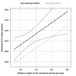
It is possible to get predicted values, together with confidence
bands for means or individuals using the |
fm <- bwt ~ lwt + smoke
new.df <- expand.grid(lwt=seq(80, 250, by=10),
                      smoke=levels(birthwt$smoke))
new.df <- data.frame(new.df, predict(lm(fm, data=birthwt),
                                     newdata=new.df,
interval="confidence")) |
|
Next, we build a rather complex plot with \docpkg{lattice} to display fitted regression line with associated 95\% confidence bands (for predicting the mean).
|
my.panel.bands <- function(x, y, upper, lower, col, subscripts, ...) {
  upper <- upper[subscripts]
  lower <- lower[subscripts]
  panel.lines(x, lower, ...)
  panel.lines(x, upper, ...)
}
my.col <- c("black", "gray60")
my.key <- simpleKey(text=c("Not smoking mother","Smoking mother"),
                    points=FALSE, col=my.col, columns=2)
xyplot(fit ~ lwt, data=new.df, groups=smoke,
       upper = new.df$upr, lower = new.df$lwr,
       xlab="Mother's weight at last menstrual period (pounds)",
       ylab="Expected birth weight (grams)",
       col=my.col, lty=1:2, key=my.key,
       panel = function(x, y, ...){
         panel.superpose(x, y, panel.groups = my.panel.bands,
                         type='l', ...)
         panel.xyplot(x, y, type=c("b","g"), cex=0.6, pch=19,
                      lwd=2, ...)})
|
|
Although not recommended because of the lack of control on p-values
or biased R2 values, we could use |
birthwt$age.s <- scale(birthwt$age, scale=F)
lm.fit7 <- lm(bwt ~ . + ht:age.s + ptl:ftv + ui:ftv,
              data=birthwt[,-1])
lm.fit7.step <- step(lm.fit7,
                     scope=list(lower= ~ smoke + ht*age.s + race,
                                upper= ~ .), trace=FALSE)
summary(lm.fit7.step) |
|
A better way to perform variable selection is through penalization, i.e. shrinkage of regression coefficients to zero or use of penalized likelihood. |
|
Dealing with categorical outcomes |
|
Comparing two proportions |
|
|
Considering the cross-classification of the existence of previous premature labours (yes/no) with number of physician visits during the first trimester (1 or more than one), we can ask whether there is any association between the two variables using a chi-square test. |
ptd <- factor(birthwt$ptl > 0, labels=c("No","Yes"))
ftv2 <- factor(ifelse(birthwt$ftv < 2, "1", "2+"))
tab.ptd.ftv <- table(ptd, ftv2)
prop.table(tab.ptd.ftv, 1)
chisq.test(tab.ptd.ftv) |
|
More association measures are available through the |
|
|
Here is a simple estimate of the odds-ratio, ignoring the stratification factor: |
library(vcd)
oddsratio(xtabs(~ low + smoke, data=birthwt), log=FALSE)
fourfold(xtabs(~ low + smoke, data=birthwt),
         color=rep(c("gray30","gray80"), 3))
tab.low.smoke.by.race <- xtabs(~ low + smoke + race, data=birthwt)
plot(oddsratio(tab.low.smoke.by.race)) |
|
Compared to stratum-specific \textsc{or}s (see below), the common estimate equals 3.09. |
with(birthwt, mantelhaen.test(low, smoke, race))
for (i in 1:3)
  print(oddsratio(xtabs(~ low + smoke,
                        data=subset(birthwt, as.numeric(race)==i)),
log=FALSE)) |
Testing association in a 2 x k Table |
|
|
Instead of using a binary indicator, we could also use a trend test which has higher power than the chi-square test when there is indeed a linear or monotonic trend. This test is equivalent to a score test for testing H0: β=0 in a logistic regression model, but it can be computed from the M2 = (n−1)r2 statistic (Agresti, 2002). |
|
|
Consider, for example, three ordered classes for number of physician
visits ( |
birthwt$ftv.c <- cut2(birthwt$ftv, c(0, 1, 2, 6))
xtabs(~ low + ftv.c, data=birthwt)
independence_test(low ~ ftv.c, data=birthwt, teststat="quad",
scores=list(ftv.c=c(0,1,4))) |
Testing association in a three-way Table |
|
|
When there are more than two variables, we need dedicated methods to
display and test associations. Everything is readily available in
the |
age.q <- cut2(birthwt$age, g=4)
structable(low ~ age.q + ftv2 + ht, data=birthwt) |
|
A more friendly visual summary using a mosaic display. |
mosaic(~ low + age.q + ftv2, data=birthwt, shade=TRUE,
       labeling_args=list(set_varnames=c(low="Weight < 2.5 kg",
                            age.q="Age range",
                            ftv2= "No. physician visits")))
|
Modeling a binary outcome |
|
Logistic regression |
|
|
One of the models discussed by Hosmer and Lemeshow was about how low
birth weight (<2.5 kg, |
|
|
Such a model can be fitted using the |
library(rms)
ddist <- datadist(birthwt)
options(datadist="ddist")
fit.glm1 <- lrm(low ~ age + lwt + race + ftv, data=birthwt)
print(fit.glm1) |
|
A summary of the effects of each factor (OR with 95\% CI) can be
obtained through the |
summary(fit.glm1) |
|
A likelihood ratio test indicates that at least one coefficients is
non zero. It appears that |
fit.glm2 <- update(fit.glm1, . ~ . - age - ftv)
lrtest(fit.glm2, fit.glm1)
anova(fit.glm2) |
|
Finally, we could predict the expected outcome (with confidence intervals for means) for a particular range of weight at last menstrual period, depending on mother’s ethnicity. |
pred.glm2 <- Predict(fit.glm2, lwt=seq(80, 250, by=10), race)
xYplot(Cbind(yhat,lower,upper) ~ lwt | race, data=pred.glm2,
method="filled bands", type="l", col.fill=gray(.95)) |
|
Still on the log odds scale, we can predict the expected weight
category for a white mother’s of last menstrual weight |
Predict(fit.glm2, lwt=150, race="White") |
|
Or we can use the regression equation directly since we have access parameters estimates. The OR is computed as: |
exp(sum(coef(fit.glm2)*c(1, 150, 0, 0))) |
What’s next? |
|
|
Model diagnostic and model selection are important steps when building a predictive model, though it was not discussed here. A very thorough review of relevant methods is available in Steyerberg (2009). |
|
Bibliography |
|
|
[1] Hosmer D, Lemeshow S. Applied Logistic Regression. New York:
Wiley; 1989. |
|
|
Last updated: Thu Oct 27 13:52:00 CEST 2011. This document has been prepared using rocco and R version 2.13.2. |
|