Fisher’s Pioneering work on Discriminant Analysis and its Impact on AI (https://arxiv.org/abs/2309.04774v1)

It’s a little bit funny to see the name of Ronald Fisher associated to AI in the title of scientific paper, especially since AI now means LLMs and other brilliant foundations for the future millennium. Anyway, the iris dataset is used to illustrate the use of a discriminant function (as the ratio of squared mean and variance) to demonstrate whether “when we use the linear compound of the four measurements most appropriate for discriminating three such species, the mean value for I. versicolor takes an intermediate value and, if so, whether it differs twice as much from I. setosa as from I. virginica, as might be expected, if the effect of genes are simply additive, in a hybrid between a diploid and a tetraploid species.” ¹ Hence, a genetic hypothesis, which can be exploited to find the optimal linear combination of population means, $\mu_1 -3\mu2 + 2\mu_3 = 0$ (respectively, setosa, versicola and virginica), was at the heart of Fisher’s seminal paper, like many of his other contributions. Sadly, the iris dataset is mostly used in the context of unsupervised classification (k-means, for instance), as if people forgot that it relies at its heart on a well-defined hypothesis (much like people forgot or still ignore that Student (Gosset’s nom de plume) developed his test while working in a brewery). It seems the point of the authors is the notion of a discriminating rule, which, when applied to AI problems, amounts to a supervised approach that aims to find a “rule to separate distinct populations, and then to use that rule (or a different classification scheme) to allocate a new observation to the given populations.”

A compendium of data sources for data science, machine learning, and artificial intelligence (https://arxiv.org/abs/2309.05682)

This article summarizes a long list of data repositories spanning a dozen or so domains (including satellite data or sports, for instance). I will keep it on hand just in case I need some dataset one day.

Demystifying Statistical Matching Algorithms for Big Data (https://arxiv.org/abs/2309.05859)

Propensity scoring is widely used in the absence of a controlled experiment, e.g. in observational studies, where as the authors say matching is used to pair treated and control units with similar value of potential confounders (aka, the propensity score). Usually, matching is done with replacement, that is a control is paired to several treated units (1-to-n matching, with replacement). There are other estimators (e.g., inverse probability weighting or doubly robust methods), though. Oversampling and replacement strategies may alter the balance between bias and variance. In the case of matching without replacement, greedy approaches are used; in Stata, there’s a command calipmatch which does the job for you, while in R the /de facto/ packages are probably Matching and MatchIt. In this paper, the authors review alternative approaches, namely optimal statistical matching (linear balanced and unbalanced assignment problem, maximum cardinality matching, and minimal cost matching).

Subgroup detection in linear growth curve models with generalized linear mixed model (GLMM) trees (https://arxiv.org/abs/2309.05862)

Here is another paper by Achim Zeilis on regression trees. This time, it deals with “extended” GLMMs for identifying subgroups in growth curve modeling. It’s been a long time since I first used partykit for tree-structured regression and classification models, and this was in a benchmark with classical CART, logic regression, and ensemble methods (random forests and boosting); this didn’t end up in a paper, but it was a fun exercise. Since then, a lot of work has been put forward into this framework and I’m not really up to date. Unlike other methods for partitioning latent growth curves, this modeling framework set up a mixed approach: “GLMM trees do not fit a full parametric model in each of the subgroups defined by the terminal nodes of the tree. Instead, fixed-effects parameters are estimated locally, using the observations within a terminal node, and the random-effects parameters are estimated globally, using all observations.”

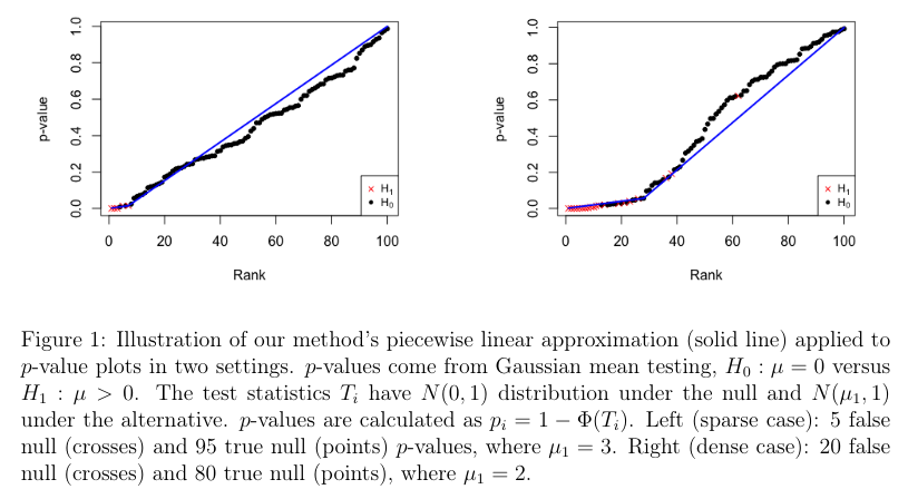
A Change-Point Approach to Estimating the Proportion of False Null Hypotheses in Multiple Testing (https://arxiv.org/abs/2309.10017)

I have used FDR correction for multiple comparisons here and there, as an alternative to sequential methods like Holm’s approach (which is the default in R’s p.adjust, btw). The authors offer an alternative data-driven method to the classical Storey’s method (i.e., a family of true null proportion of false null hypotheses estimators) for estimating the FDR. In this case, the sorted p-values are approximated using a piecewise linear function with one change point (inversion of slope), as illustrated below. This is somewhat akin to the knee/elbow method or scree plots for determining the number of principal components or factors to retain in PCA or FA, which is discussed in section C.1.

A New Bootstrap Goodness-of-Fit Test for Normal Linear Regression Models (https://arxiv.org/abs/2309.10614)

Yet another article discussing the benefit of using bootstrap to assess model goodness-of-fit. Rather than visual inspection of so-called residual plots (residuals vs. fitted values), especially in multivariate regression, or relying on either the White or Breusch-Pagan test. The test presented here allows to test all assumptions of normal linear regression:

For test level $\alpha$, candidate normal linear model $\mathcal{M}$, bootstrap iterations $B$, sample size $n$, and a null hypothesis that $\mathcal{M}$ is adequately specified:

1. Resample, with replacement, outcomes with covariates to generate a bootstrap sample of size $n$.
2. Fit model $\mathcal{M}$ to this bootstrap sample, and with this fitted model, calculate $\text{Var}[\text{GOF}]$and record this statistic.
3. Repeat steps 1-2 $B$ times to generate an empirical bootstrap distribution for $\text{Var}[\text{GOF}]$.
4. Construct a $100\times (1−\alpha)$% bootstrap confidence interval for $\text{Var}[\text{GOF}]$.
5. If this interval does not contain $2n$, reject the null hypothesis at the $\alpha$ level. If it does contain $2n$, the null hypothesis was not rejected and model $\mathcal{M}$ does not appear to exhibit lack-of-fit.

Unveiling Challenges in Mendelian Randomization for Gene-Environment Interaction (https://arxiv.org/abs/2309.12152)

As a sequel to this 10-years old post, here is a paper that uses genetic variants as instrumental variables (2-stage predictor substitution and the 2-stage residual inclusion) to estimate causal effects in GWAS on lifestyle and environmental factors.