Capture-recapture sampling
Capture-recapture (CR) sampling is widely used in ecological research, epidemiology and population biology. I saw a tweet a few days ago that nicely illustrates the CR method using animated graphics, which has been followed by a blog post since then.
The basic idea underlying CR sampling is that you use simple random sampling to capture a set of n individuals out of a population of size N, release this sample once all items have been marked, and then iterate. Sample sizes do not necessarily have to be identical among each capture stage, but you must assume that marking does not affect survival, and that the population is fixed (no death, no new individual). Suppose you take a first sample of size 10 and a second sample of size 15, of which 5 were already marked during the first stage, then the estimated population size would be (10 x 15) / 5 = 30. Obviously, the smaller the number of recaptures, the larger the estimate of population size will be, which makes sense if we think in term of measuring abundance of some quantity. How do we found this number? Assume that x denotes the number of marked individuals in the observed sample, and X the corresponding marked individuals in the population of size N. Then, assuming that the population and sample proportions are equal, i.e., x/n = X/N, we have N = Xn/x. This is known as the Lincoln-Peterson Index.1
Another way to show this is to consider the following cross-classification table, where captured individuals are in columns and recaptured indivudals in rows:2
| Yes | No | Total | |
|---|---|---|---|
| Yes | a | b | a+b |
| No | c | x | |
| Total | a+c | N = a+b+c+d |
Assuming the capture and recapture stage are independent, the estimated probability of being captured on both occasions is equal to the product of the probabilities of being captured on each occasion. The missed individuals, x, is then computed as follows: $\frac{a}{N} = \left( \frac{a+c}{N}\right)\times \left( \frac{a+b}{N}\right)$, whence $a(a+b+\hat x) = (a+c)(a+b)$ and $\hat x = \frac{bc}{a}$.
This of course is the hypergeometric distribution in disguise. The hypergeometric distribution plays a central role in random sampling with finite populations. Let’s consider an urn with red and black balls. Each time you draw a ball, without replacement: what’s the probability of drawing n red balls? Unlike the case of the binomial distribution, each drawing stage influence the outcome of the next draw since the ratios of red to black balls changes after each draw. Now let’s replace red balls with marked individuals from the preceding paragraph, and let’s call it Y the number of individuals that were marked. The probability function of Y reads:
$$ \Pr(Y = y) = \frac{{X \choose N}{N-X \choose n-x}}{{N \choose n}}, $$
such that the value Xn/x shown above corresponds to the maximum likelihood estimate of N (write up P(N)/P(N-1) and find N such that P(N-1) < P(N)).
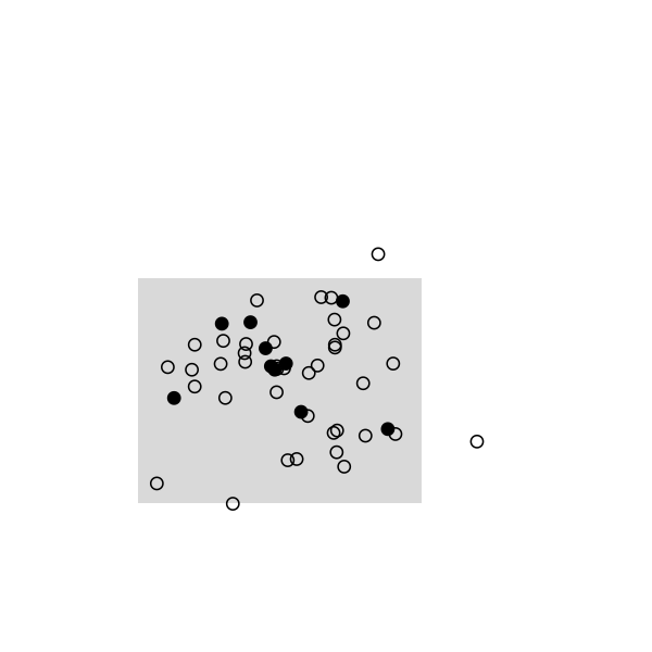
Here are some highlights from a small simulation in R. I used a 2D random walk to animate a population of 50 individuals, which were sampled once every 20 frames (sampling rate, 10/50). This baiscally looks like this in R:
walker <- function(n, step = 0.1) {
  coord <- replicate(2, sample(c(-1, 1), n, rep = TRUE) + step * rnorm(n))
  return(apply(coord, 2, cumsum))
}
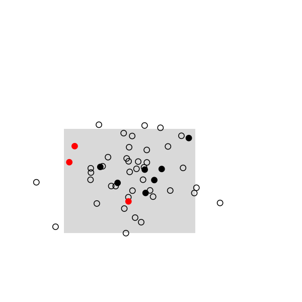
The remaining of the script is a simple loop to draw the main frame and select randomly 10 individuals every 20 frames. The size and position of the rectangle of sampling ensures that we see enough individuals, but it can be changed. Selected individuals are marked in black, and those who were marked at the preceding stage are highlighted in red. Ideally, we should observe 2 recaptures to recover the exact population size, (10 x 10) /2:
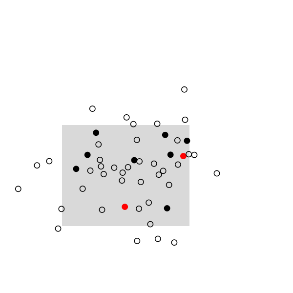
And the full story:
Since this index is sensitive to the number of recapture, another index has been proposed, the Schnabel index (note that it also depends on the number of CR stages). ↩︎
Tlling, Kate. Capture-recapture methods—useful or misleading? International Journal of Epidemiology 2001, 30: 12–14. ↩︎