Usually, we would determine the number of permutations required to carry out a Monte Carlo permutation test based on the precision we wish to attain for the p-value. In fact, Stata provides a confidence interval for the estimated p-value when you use the permute procedure. This confidence interval is based on a binomial proportion (this is what we are estimating after all). With the example discussed in a previous post, converted as a tabular dataset, here is a sample run from Stata 13:

. insheet using how-many-permutations.csv
. gen i=_n
. reshape long v, i(i)
. permute _j r(mu_1), reps(10000): ttest v, by(_j)
// -%----
Monte Carlo permutation results                   Number of obs   =         20

      command:  ttest v, by(_j)
        _pm_1:  r(mu_1)
  permute var:  _j

------------------------------------------------------------------------------
T            |     T(obs)       c       n   p=c/n   SE(p) [95% Conf. Interval]
-------------+----------------------------------------------------------------
       _pm_1 |      14.48    5229   10000  0.5229  0.0050   .513055   .5327317
------------------------------------------------------------------------------
Note:  Confidence interval is with respect to p=c/n.
Note:  c = #{|T| >= |T(obs)|}

Note that we get a p-value close to the one estimated using Lisp or R. It is also possible to carry out an exact permutation test using the enumerate option. Philip Good provides illustrations with various statistical software in chapter 3 of one of his textbook.¹

The approximate 95% CI for a proportion estimated from a sample of size $n$ is

$$ \hat p \pm 2\sqrt{\frac{\hat p(1-\hat p}{n}}, $$

which can be approximated as $\hat p \pm \sqrt{\hat p/n}$ for small $\hat p$. As an example, to get a precision of two decimal places for a proportion of 0.01, we would need $n > 1600$ rearrangements ($0.01 > 4\sqrt{0.01/n}$, then solve for $n$). This is probably why the rule of thumb is to use 1000 to 10000 permutations, when not “use the maximum number of permutations”. Of course, this only applies to Monte Carlo re-rerandomization, since in the case of exact permutation tests you get the “exact” p-value you get, which is tied to your sample size. E.g., with five observations you only have 32 possibilities and 1 extreme observation out of 32 means a p-value of 0.03125.²

And here is yet another way to carry out a permutation test, although it is suboptimal (in many ways). This time, we will simply shuffle the whole sequence of observation and take the first half part of the sequence. Again, we will rely on a Monte Carlo approach and only carry out a limited number of random draws from the original sample. Last but not least, we will replace Scheme with Clojure.

As before, we will consider the sum of the observations in one group (the original, then the randomized one) as our test statistic. Other solutions such as taking the difference in means or the detrended Student t statistic are also possible.

(def xs [12.9 13.5 12.8 15.6 17.2 19.2 12.6 15.3 14.4 11.3])
(def ys [12.7 13.6 12.0 15.2 16.8 20.0 12.0 15.9 16.0 11.1])
(def xy (concat xs ys))
(def stat0 (apply + xs))
(def k 1000)
(defn stat [x] (apply + (take 10 (shuffle x))))
(def pdist (repeatedly k (partial stat xy)))
(def events (count (filter (fn [x] (> x stat0)) pdist)))
(double (/ events k))
;; => 0.525

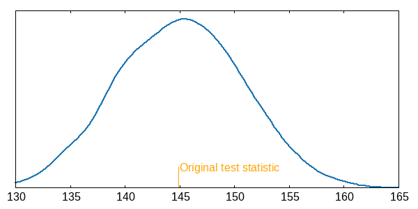
Run time is quite decent in this case, even for large k. Now let’s check the distribution of the permuted test statistic? Here’s one with 10000 iterations (p=0.5156) and the venerable Gnuplot backend.³

set terminal png size 600, 300
set output "~/tmp/pdist.png"
set xrange [130:165]
set yrange [0:7]
unset key
unset ytics
set arrow 1 from 144.8,0 to 144.8,0.8 lc "orange" nohead
set label "Original test statistic" at 145,0.75 tc "orange"
plot "pdist.dat" u 1:(1/100.) s kdens bandwidth 1 lw 2

Overall, I was pleasantly surprised by how easy it was to perform this task in Clojure by using builtin stuff only.