Computing intraclass correlation with R
I always found Dave Garson’s tutorial on Reliability Analysis very interesting. However, all illustrations are with SPSS. Here is a friendly R version of some of these notes, especially for computing intraclass correlation.
Background
They are different versions of the intraclass correlation coefficient (ICC), that reflect distinct ways of accounting for raters or items variance in overall variance, following Shrout and Fleiss (1979) cases 1 to 3 in Table 1):
- One-way random effects model: each item is rated by different raters who are considered as sampled from a larger pool of potential raters, hence they are treated as random effects; the ICC is then interpreted as the % of total variance accounted for by subjects/items variance. This is called the consistency ICC.
- Two-way random effects model: both factors–raters and items/subjects–are viewed as random effects, and we have two variance components (or mean squares) in addition to the residual variance; we further assume that raters assess all items/subjects; the ICC gives in this case the % of variance attributable to raters + items/subjects.
- Two-way mixed model: contrary to the one-way approach, here raters are considered as fixed effects (no generalization beyond the sample at hand) but items/subjects are treated as random effects; the unit of analysis may be the individual or the average ratings.
They are called ICC(1,1), ICC(2,1), and ICC(3,1) when we have only one rating for each rater x item combination, and ICC(1,k), ICC(2,k), and ICC(3,k) when the reported rater x item cell is an average.
Computing ICC with R
There are many ways to get ICC estimates, including psy (icc), psych (ICC), or irr (icc). I will use the latter one.
I fetched the data from here , which looks like a general repository for SPSS example dataset that I don’t have. Let’s go with the tv-survey.sav dataset which D. Garson used when describing ICC. Quoting his words:
Some 906 respondents were asked if they would watch a particular show for….
- Any reason
- No other popular shows on at that time
- Critics still give the show good reviews
- Other people still watch the show
- The original screenwriters stay
- The original directors stay
- The original cast stays
where answers were coded 0=No or 1=Yes.
I happened to load the data and recode them as binary variable as follows:
> library(foreign)
> tv <- read.spss("tv-survey.sav", to.data.frame=T)
> head(tv)
  ANY BORED CRITICS PEERS WRITERS DIRECTOR CAST
1  N0    NO      NO    NO     YES      YES  YES
2 YES   YES      NO   YES     YES      YES  YES
3 YES   YES     YES   YES     YES      YES  YES
4 YES   YES     YES   YES     YES      YES  YES
5 YES   YES     YES   YES     YES      YES  YES
6 YES   YES     YES   YES     YES      YES  YES
> dim(tv)
[1] 906   7
> tv.num <- sapply(tv, function(x) as.numeric(x)-1)
Then, computing ICC for “Singles Measures” is just a matter of running:
> library(irr)
> icc(t(tv.num))
 Single Score Intraclass Correlation

   Model: oneway
   Type : consistency

   Subjects = 7
     Raters = 906
     ICC(1) = 0.143

 F-Test, H0: r0 = 0 ; H1: r0 > 0
  F(6,6335) = 152 , p = 8.02e-181

 95%-Confidence Interval for ICC Population Values:
  0.064 < ICC < 0.448
The default settings correspond to the so-called “consistency” ICC, that is ICC computed from a one-way ANOVA where raters are considered as random effects (henece, representative of a larger pool of raters). But D. Garson also showed ICC for “Average measures”, which means that we consider the unit of analysis to be the mean of several ratings. This is readily obtained using the following instruction:
> icc(t(tv.num), unit="average")
 Average Score Intraclass Correlation

   Model: oneway
   Type : consistency

   Subjects = 7
     Raters = 906
   ICC(906) = 0.993

 F-Test, H0: r0 = 0 ; H1: r0 > 0
  F(6,6335) = 152 , p = 8.02e-181

 95%-Confidence Interval for ICC Population Values:
  0.984 < ICC < 0.999
However, in this particular case, it doesn’t apply (or it is not obvious from the description of the data that ratings can be regarded as average ratings).
Tukey non-additivity test
Dave Garson mentioned the use of Tukey non-additivity test for checking the assumption of no raters by items interaction. I must admit I never used it in this situation. I didn’t find any references in Dunn’s textbook on the Design and Analysis of Reliability Studies (Oxford Univ. Press, 1989). A little googling didn’t reveal any recent application of this test in the context of reliability studies, but I did find a paper that discusses its validity [1]. It should be noted that we are in the case of a single rating/item, that is there’re no repetitions in the ratings which prevent from estimating an interaction effect from the ANOVA table (at least, the interaction term is confoudned with the error term). Moreover, it only applies to the case 2 and 3 above, where we can form a two-way model (raters x items).
Hopefully, this test is available in the agricolae package as nonadditivity(). I tested it against Stata nonadd command and got the same results:
. findit nonadd
. use https://stats.idre.ucla.edu/stat/stata/faq/rb4a, clear
(RB Example - Kirk, 1982)
. anova y a s

                           Number of obs =      32     R-squared     =  0.8790
                           Root MSE      = 1.16496     Adj R-squared =  0.8214

                  Source |  Partial SS    df       MS           F     Prob > F
              -----------|----------------------------------------------------
                   Model |         207    10        20.7      15.25     0.0000
                         |
                       a |       194.5     3  64.8333333      47.77     0.0000
                       s |        12.5     7  1.78571429       1.32     0.2914
                         |
                Residual |        28.5    21  1.35714286
              -----------|----------------------------------------------------
                   Total |       235.5    31  7.59677419

. nonadd y a s

Tukey's test of nonadditivity (Ho: model is additive)
SS nonadd = 8.0218509  df = 1
F (1,20) = 7.8345468   Pr > F: .01108091
In R, using the file rb4a.dat, we have:
> rb4a <- read.table("rb4a.dat", header=T, colClasses=c("numeric","factor","factor"))
> summary(aov(y ~ ., rb4a))
            Df Sum Sq Mean Sq F value    Pr(>F)
a            3  194.5  64.833 47.7719 1.478e-09 ***
s            7   12.5   1.786  1.3158    0.2914
Residuals   21   28.5   1.357
---
Signif. codes:  0 ‘***’ 0.001 ‘**’ 0.01 ‘*’ 0.05 ‘.’ 0.1 ‘ ’ 1
> lm0 <- lm(y ~ ., data=rb4a)
> df.lm0 <- df.residual(lm0)
> MSE.lm0 <- deviance(lm0)/df.lm0
> res <- with(rb4a, nonadditivity(y, a, s, df.lm0, MSE.lm0))

Tukey's test of nonadditivity
y

P : -49.375
Q : 303.9062

Analysis of Variance Table

Response: residual
              Df  Sum Sq Mean Sq F value  Pr(>F)
Nonadditivity  1  8.0219  8.0219  7.8345 0.01108 *
Residuals     20 20.4781  1.0239
---
Signif. codes:  0 ‘***’ 0.001 ‘**’ 0.01 ‘*’ 0.05 ‘.’ 0.1 ‘ ’ 1
It is important not to forget to treat a and s as factors. Let’s see it in action:
> library(reshape)
> tv.num.t.long <- melt(t(tv.num))
> tv.num.t.long$X2 <- factor(tv.num.t.long$X2)
> library(agricolae)
> lm0 <- lm(value ~ X1 + X2, data=tv.num.t.long)
> df.lm0 <- df.residual(lm0)
> MSE.lm0 <- deviance(lm0)/df.lm0
> res <- with(tv.num.t.long, nonadditivity(value, X1, X2, df.lm0, MSE.lm0))
Tukey's test of nonadditivity
value

P : -76.04803
Q : 89.38298

Analysis of Variance Table

Response: residual
                Df Sum Sq Mean Sq F value    Pr(>F)
Nonadditivity    1  64.70  64.703  845.95 < 2.2e-16 ***
Residuals     5429 415.24   0.076
---
Signif. codes:  0 ‘***’ 0.001 ‘**’ 0.01 ‘*’ 0.05 ‘.’ 0.1 ‘ ’ 1
Ok, so we see that there’s a significant linear item by linear rater interaction.
As an example of random blocks without interaction, let’s consider data from Table 2 in Lahey et al’s paper, which comes from Shrout & Fleiss’s original paper in 1979:
> tab2 <- matrix(c(9,6,8,7,10,6,
                   2,1,4,1,5,2,
               5,3,6,2,6,4,
               8,2,8,6,9,7), nc=4)
> tab2.df.long <- melt(tab2, varnames=c("Target","Judge"))
> tab2.df.long$Target <- factor(tab2.df.long$Target)
> tab2.df.long$Judge <- factor(tab2.df.long$Judge)
> lm0 <- lm(value ~ ., data=tab2.df.long)
> df.lm0 <- df.residual(lm0)
> MSE.lm0 <- deviance(lm0)/df.lm0
> res <- with(tab2.df.long, nonadditivity(value, Target, Judge, df.lm0, MSE.lm0))


Tukey's test of nonadditivity
value

P : 15.58681
Q : 912.9951

Analysis of Variance Table

Response: residual
              Df  Sum Sq Mean Sq F value Pr(>F)
Nonadditivity  1  0.2661  0.2661  0.2479 0.6263
Residuals     14 15.0256  1.0733
Tukey’s test here confirms that there’s no interaction. To find the corresponding ICC(3,1) given by Shrout and Fleiss (1979), we need to use a two-way model:
> icc(tab2, model="twoway")
 Single Score Intraclass Correlation

   Model: twoway
   Type : consistency

   Subjects = 6
     Raters = 4
   ICC(C,1) = 0.715

 F-Test, H0: r0 = 0 ; H1: r0 > 0
    F(5,15) = 11 , p = 0.000135

 95%-Confidence Interval for ICC Population Values:
  0.342 < ICC < 0.946
The second example discussed by Lahey et al. include an interaction effect (the last column from Table 2 was changed to negatively correlate with the others). Let’s go with it:
> tab4 <- matrix(c(9,6,8,7,10,6,
                   2,1,4,1,5,2,
           5,3,6,2,6,4,
           3,9,3,5,2,4), nc=4, dimnames=list(1:6, 1:4))
> tab4.df.long <- melt(tab4, varnames=c("Target","Judge"))
> tab4.df.long$Target <- factor(tab4.df.long$Target)
> tab4.df.long$Judge <- factor(tab4.df.long$Judge)
> lm0 <- lm(value ~ ., data=tab4.df.long)
> df.lm0 <- df.residual(lm0)
> MSE.lm0 <- deviance(lm0)/df.lm0
> res <- with(tab4.df.long, nonadditivity(value, Target, Judge, df.lm0, MSE.lm0))


Tukey's test of nonadditivity
value

P : 2.246528
Q : 155.9048

Analysis of Variance Table

Response: residual
              Df Sum Sq Mean Sq F value Pr(>F)
Nonadditivity  1  0.032  0.0324  0.0075 0.9321
Residuals     14 60.259  4.3042
There’s no effect of Target, as can be seen in the ANOVA Table:
> anova(lm0)
Analysis of Variance Table

Response: value
          Df Sum Sq Mean Sq F value   Pr(>F)
Target     5 11.208  2.2417  0.5577 0.730692
Judge      3 83.458 27.8194  6.9212 0.003802 **
Residuals 15 60.292  4.0194
---
Signif. codes:  0 ‘***’ 0.001 ‘**’ 0.01 ‘*’ 0.05 ‘.’ 0.1 ‘ ’ 1
To fully reproduce Lahey et al’s Tabel 5, the missing MS (within targets) might be obtained as follows:
> unlist(summary(aov(value ~ Target, data=tab4.df.long)))["Mean Sq2"]
Mean Sq2
7.986111
(By the way, there is a typo in Lahey et al’s Table 5: the corresponding DF for the between targets effect should read 5, not 3.)
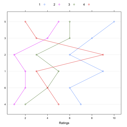
Now, what’s interesting is that the ICC is negative, but Tukey’s test failed to recover the significant interaction, while clearly Rater 4 is at variance with others’ ratings:
> round(cor(tab4), 2)
      [,1]  [,2]  [,3]  [,4]
[1,]  1.00  0.75  0.73 -0.75
[2,]  0.75  1.00  0.89 -0.73
[3,]  0.73  0.89  1.00 -0.72
[4,] -0.75 -0.73 -0.72  1.00
This might also be shown visually, where Target have been reordered by their mean rating:
> library(lattice)
> dotplot(tab4[order(apply(tab4, 1, mean)),], type="b")
In conclusion, the characteristic root test of the interaction might provide an interesting alternative to Tukey’s test when there’s no main effect [2,3]. I’m not aware of any available R implementation. I should write one. Other relevant papers are listed in the References below.
References
- Lahey, M.A., Downey, R.G., and Saal, F.E. (1983). Intraclass Correlations: There’s More There Than Meets the Eye. Psychological Bulletin, 93(3), 586-595.
- Johnson, D.E. and Graybill, F.A. (1972). An analysis of a two-way model with interaction and no replication. Journal of the American Statistical Association, 67, 862-868.
- Hegemann, V. and Johnson, D.E. (1976). The power of two tests for nonadditivity. Journal of the American Statistical Association, 71(356), 945-948.
- Alin, A. and Kurt, S. (2006). Testing non-additivity (interaction) in two-way ANOVA tables with no replication. Statical Methods in Medical Research, 15, 63-85.
- Rasch, D. et al. (2008). Tests of additivity in mixed and fixed effects two-way ANOVA models with single subclass numbers. The International Conference on Trends and Perspectives in Linear Statistical Inference. Będlewo, Poland.
- Šimečková, M., Šimeček, P., and Rasch, D. (2008). Test of additivity in two-way ANOVA models with single subclass numbers. Robust.
- McGraw, K.O. and Wong, S.P. (1996). Forming Inferences About Some Intraclass Correlation Coefficients. Psychological Methods, 1(1), 30-46.
- Bartko, J.J. (1976). On Various Intraclass Correlation Reliability Coefficients. Psychological Bulletin, 83(5), 762-765.
Sidenote
For the second dataset, the SAV file I used was GSS93_subset.sav. and I happened lo load it into R as follows:
> gss <- read.spss("GSS93 subset.sav", to.data.frame=T)
> items.idx <- 10:13
> gss.it <- gss[,items.idx]
> gss.it.num <- sapply(gss.it, function(x) as.numeric(x))
Then, to compute Cronbach’s alpha and item-scale statistics, I used:
> library(psych)
> alpha(gss.it.num)
This gives:
 raw_alpha std.alpha G6(smc) average_r mean  sd
       0.7      0.79    0.82      0.49  4.7 1.4

Reliability if an item is dropped:
       raw_alpha std.alpha G6(smc) average_r
EDUC        0.68      0.69    0.62      0.43
DEGREE      0.53      0.71    0.63      0.45
PADEG       0.66      0.78    0.78      0.54
MADEG       0.68      0.78    0.79      0.54

Item statistics
          n    r r.cor r.drop mean   sd
EDUC   1496 0.84  0.84   0.71 13.0 3.07
DEGREE 1496 0.83  0.82   0.81  2.4 1.18
PADEG  1207 0.74  0.59   0.48  1.9 1.19
MADEG  1352 0.73  0.58   0.48  1.8 0.94
This is in close agreement with the results reported by Dave Garson. Now, fitting an ANOVA model and applying the Tukey’s test yields:
> gss.it.num.long <- melt(gss.it.num)
> gss.it.num.long$X1 <- factor(gss.it.num.long$X1)
> lm0 <- lm(value ~ ., data=gss.it.num.long)
> anova(lm0)
However, since there are missing responses, let’s do the analysis by considering complete cases only. Testing for nonadditivity then yields the following results:
Tukey's test of nonadditivity
value

P : 51572.02
Q : 734728.4

Analysis of Variance Table

Response: residual
                Df Sum Sq Mean Sq F value    Pr(>F)
Nonadditivity    1 3619.9  3619.9  3793.8 < 2.2e-16 ***
Residuals     3368 3213.7     1.0
---
Signif. codes:  0 ‘***’ 0.001 ‘**’ 0.01 ‘*’ 0.05 ‘.’ 0.1 ‘ ’ 1
Again, this is pretty close to what Dave Garson reported on his website, with the right degrees of freedom. The syntax used for obtaining the above result was:
> gss.it.num.long.noNA <- melt(na.omit(gss.it.num))
> gss.it.num.long.noNA$X1 <- factor(gss.it.num.long.noNA$X1)
> lm0 <- lm(value ~ ., data=gss.it.num.long.noNA)
> df.lm0 <- df.residual(lm0)
> MSE.lm0 <- deviance(lm0)/df.lm0
> res <- with(gss.it.num.long.noNA, nonadditivity(value, X1, X2, df.lm0, MSE.lm0))