Interaction terms in nonlinear models
This discussion is primarily based on the following article, but see also:(1,2) Ai, C. and Norton, E.C. (2003). Interaction terms in logit and probit models. Economics Letters, 80: 123-129.
The magnitude of the interaction effect in nonlinear models does not equal the marginal effect of the interaction term, can be of opposite sign, and its statistical significance is not calculated by standard software. We present the correct way to estimate the magnitude and standard errors of the interaction effect in nonlinear models.
The main ideas of this article is that both the test and interpretation of an interaction term in a GLM are done in the wrong way. Instead of interpreting the true interaction coefficient, discussion often relies on the marginal effect of the interaction term. What are marginal effect? In this context, it means that an interaction between two factors should be combined with the main effects marginal to that interaction.(6,8) Using the notation of the authors, the interaction effect is the cross derivative of the expected value of $y$:
$$ \frac{\partial \Phi(\cdot)}{\partial x_1 \partial x_2} = \underbrace{\beta_{12}\Phi’(\cdot)}_{\text{marginal effect}} \hskip-2ex + (\beta_1 + \beta_{12})(\beta_2 + \beta_{12}x_1)\Phi’’(\cdot). $$
If $\beta_{12} = 0$, we have
$$ \frac{\partial^2 \Phi(\cdot)}{\partial x_1 \partial x_2}\Bigr|_{\substack{\beta_{12}=0}} = \beta_1\beta_2\Phi’’(\cdot). $$
In addition, the authors highlight the fact that the interaction effect might be not negligible even if the corresponding $\beta = 0$. Further, the interaction effect is conditional on the independent variables. Finally, the sign of the interaction term does not necessarily indicate the sign of the interaction effect as it may have different signs for different values of the covariates. Altogether, these remarks should give support to the practitioner so that a careful examination of the model fit is done before concluding or interpreting the interaction effect without caution.
What’s about the computation of the odds-ratio associated to the main effects when the interaction is significant? For instance, consider a logistic framework with two main effects, say $\beta_1$ and $\beta_2$ and a third coefficient $\beta_{12}$ that represents the interaction. For the purpose of the illustration, we can easily imagine two such factors, e.g., the smoking status (smoker or not) and the drinking status (occasional vs. regular drinker). The response variable might be any medical outcome of potential interest (cancer, malignant affection, etc.), coded as a binary (0/1) variable. If the interaction is significant, then talking about the odds-ratio (OR) associated to the smoking variable has no sense at all. Instead, one must describe two OR: the OR for subjects who are smoker but occasional drinker, $\exp(\beta_1)$ and the OR for subjects who are smoker and regular drinker, $\exp(\beta_1 + \beta_{12})$.
The two authors hold the necessary Stata code on their homepage. However, I would like to illustrate the issues raised by the interpretation of interaction terms when using non-linear models with R.
The effects package facilitates in some way the graphical display of effects sizes and we will use it in the short application proposed in the next few paragraphs.
Let’s consider the Arrests data, which is also used in (5) (See also this brief report, and (9), Chap. II.2, p. 57) and aims at studying the probability of release of individuals arrested in Toronto for simple possession of small quantities of marijuana. Characteristics of interest are: race, age, employment, citizenship, previous recording in police databases.
data(Arrests)
opar <- par(mfrow=c(2,2),las=1)
quali.var <- c(2,5,6,7)
for (i in quali.var)
  barplot(table(Arrests$released,Arrests[,i]),col=c(2,4),
          ylim=c(0,4000),xlab=colnames(Arrests)[i])
legend("topleft",c("Yes","No"),pch=15,col=c(2,4),bty="n",
       title="Released")
par(opar)
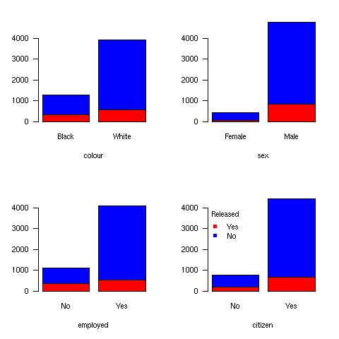
The above figure could hardly be interpreted as is because we need to consider both marginal (not shown) and conditional (these plots) distributions at the same time. However, we can run a reduced (compared to that used in (5)) model including color, age and sex, as well as color × age. This is done as follows:
arrests.glm <- glm(released ~ colour + age + sex + colour:age,
                   family=binomial, data=Arrests)
summary(arrests.glm)
and here is the resulting output:
| Effect | Estimate | Std. Error | z value | Pr(>|z|) |
| (Intercept) | 0.853219 | 0.241020 | 3.540 | 0.0004 ** |
| colourWhite | 1.645338 | 0.241690 | 6.808 | 9.92e-12 ** |
| age | 0.014389 | 0.007822 | 1.839 | 0.0658 . |
| sexMale | -0.161870 | 0.142805 | -1.133 | 0.2570 |
| colourWhite:age | -0.037299 | 0.009362 | -3.984 | 6.78e-05 ** |
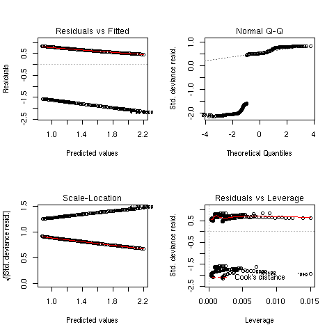
At first glance, the model seems quite satisfactory and no deviations from standard assumptions are noticed (see next Figure, left).

Now, we can get an ANOVA-like summary by issuing:(5)
library(car)
Anova(arrests.glm)
The results are shown below (see also figure above, right):
Anova Table (Type II tests)
Response: released
           LR Chisq Df Pr(>Chisq)
colour       81.854  1  < 2.2e-16
age           5.947  1    0.01474
sex           1.325  1    0.24962
colour:age   16.479  1  4.918e-05
Note that the vertical axis is labelled on the probability scale (i.e., the response scale) while the estimated effects are plotted on the scale of the linear predictor. The 95% (pointwise) confidence interval is wider at the extreme values of the age variable. Now, we can proceed to the estimation of the interaction effect using the method proposed by Ai and Norton.
References
- Ai, C. and Norton, E.C. (2000). Interaction terms in nonlinear models. Unpublished draft manuscript.
- Norton, E.C., Wang, H., and Ai, C. (2004). Computing interaction effects and standard errors in logit and probit models. The Stata Journal, 4(2), 154-167.
- Hoetker, G. (2003). Confounded coefficients: Accurately comparing logit and probit coefficients across groups. College of Business Working Papers, University of Illinois.
- Berry, W.D., Esarey, J., and Rubin, J.H. (2007). Testing for interaction in binary logit and probit models: Is a product term essential? Working Papers of the Society for Political Methodology.
- Fox, J. (2003). Effect displays in R for generalized linear models.* Journal of Statistical Software*, 8(15), 18 pp.
- Fox, J. (1987). Effect displays for generalized linear models. In Clogg, C.C. (Ed.), Sociological Methodology 1987, pp. 347-361. American Sociological Association, Washington DC.
- Rabe-Hesketh, S., Skrondal, A., and Pickles, A. (2001). Maximum likelihood estimation of generalized linear models with covariate measurement errors. The Stata Journal, 1(1), 26 pp.
- Bouyer, J., Hémon, D., Cordier, S., Derriennic, F., Stücker, I., Stengel, B., and Clavel, J. (1995). Épidémiologie, Principes et méthodes quantitatives. Éditions INSERM.
- Chen, C.-H., Härdle, W., and Unwin, A. (Eds.) (2008). Handbook of Data Visualization. Springer Verlag.
- Tomz, M., Wittenberg, J., and King, G. (2003). Clarify: Software for interpreting and presenting statistical results. Journal of Statistical Software, 8(1), 29 pp.