There are many ways to generate random samples from a given distribution, including Monte Carlo simulation. In this case, the random number generation process consists in generating i.i.d. uniform $\mathcal{U}(0,1)$ RVs, convert them to independent $\mathcal{N}(0,1)$ RVs, and eventually convert them to correlated $\mathcal{N}(0,1)$ RVs. Once we get uniform random variables on $(0,1)$, we can use one of the following methods to convert them to gaussian RVs: the Box-Muller or the Marsaglia polar method, or the inverse CDF transformation.

Regarding the Box-Muller approach the idea is as follows: You generate two independent $\mathcal{U}(0,1)$ RVs on $(0,1)$ and then you define two new independent $\mathcal{N}(0,1)$ RVs, $x_1$ and $x_2$, using this transformation:

$$ \begin{equation} \begin{aligned} x_1 &= \sqrt{-2\log(y_1)}\; \text{cos}(2\pi y_2)\cr x_2 &= \sqrt{-2\log(y_1)}\; \text{sin}(2\pi y_2). \end{aligned} \end{equation} $$

To get ride of the trigonometric functions, the Marsaglia’s polar method instead considers two independent $\mathcal{U}(0,1)$ RVs on $(-1,1)$ and accept them if $r^2 = y_1^2 + y_2^2 < 1$.¹ Once accepted, generate $x_1$ and $x_2$ as follows:

$$ \begin{equation} \begin{aligned} x_1 &= \sqrt{-2\log(r^2)/r^2}\; y_1\cr x_2 &= \sqrt{-2\log(r^2)/r^2}\; y_2. \end{aligned} \end{equation} $$

Finally, the inverse CDF transformation is a little more involved. Recall that a standard gaussian variate $Z$, with mean 0 and variance 1, has the following probability density function (PDF):

$$ \phi(z) = \frac{1}{\sqrt{2\pi}}\exp\left(-\frac{1}{2}z^2\right). $$

Its cumulative distribution function (CDF) is then $\Phi(z) = \Pr(Z<z) = \int_{-\infty}^z\phi(s)ds$. The inverse CDF method is used to compute $x = \Phi^{-1}(y)$, with $y$ distributed uniformly on $(0,1)$.

Note that the normal CDF $\Phi(x)$ is related to the error function $\text{erf}(x)$, as discussed on Wikipedia. Indeed, $\Phi(x) = \frac{1}{2} + \frac{1}{2}\text{erf}(x/\sqrt{2})$, which implies:

$$ \Phi^{-1}(y) = \sqrt{2}\;\text{erf}^{-1}(2y-1). $$

If your programming language provides you with either an inverse erf or normal CDF, then you can generate a sequence of random normal deviates easily. Here is an example using Racket:

(require math/distributions)
(define (replicate f times)
  (for ([x (in-range times)])
    (displayln (f))))
(define (rnorm [mean 0.0] [sd 1.0])
  (let ([x (random)])
    (flnormal-inv-cdf mean sd x #f #f)))
(replicate rnorm 10)

Note that Racket’s random produces random variates in the open interval $(0,1)$. If you need to include 0 and 1, for whatever reason, checkout soegaard’s answer on SO.

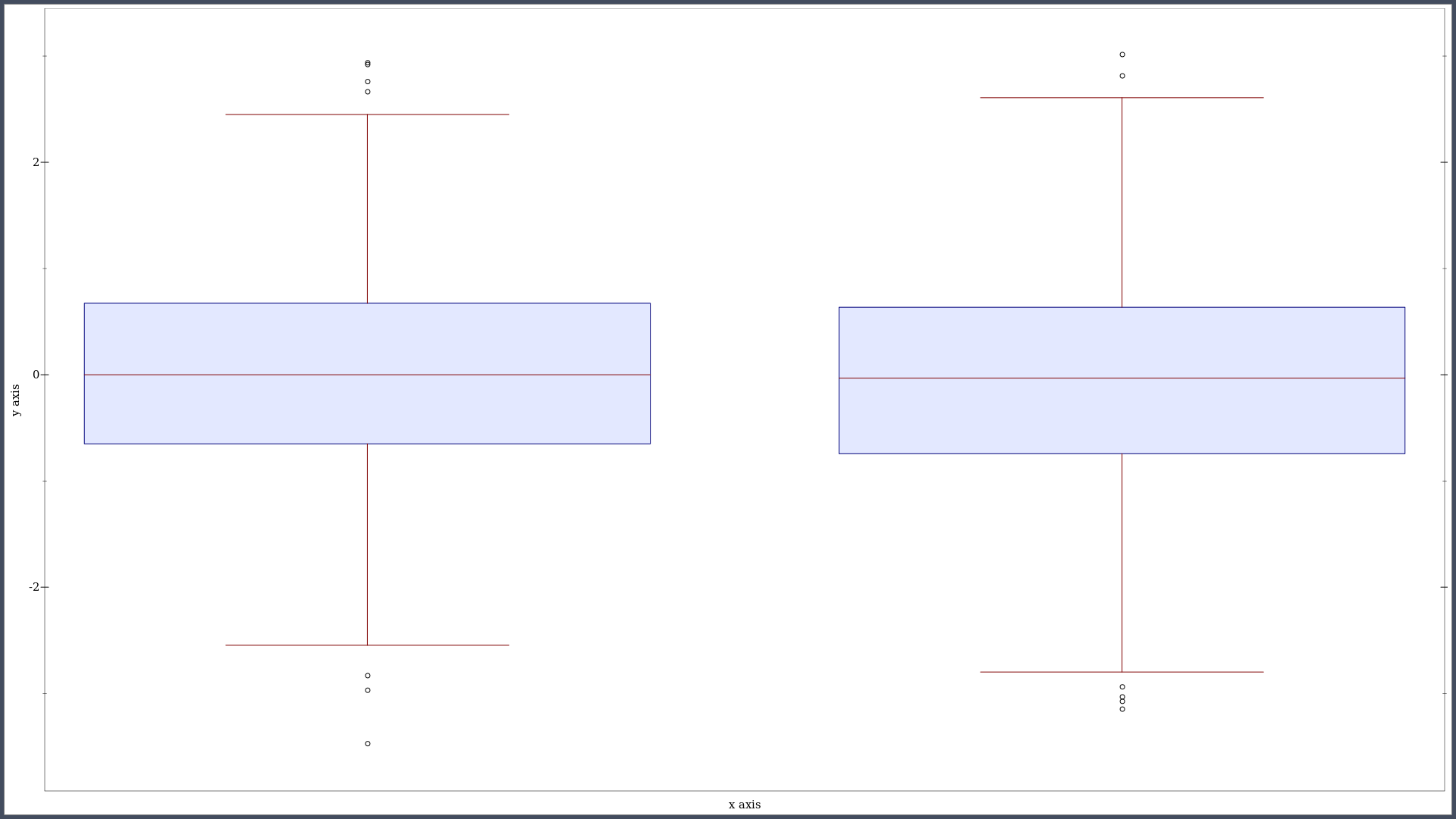
And here are two random samples of size 1000, depicted using a boxplot: (I yet have to write a quantile-quantile renderer for Racket’s plot.)

(require plot)
(plot-new-window? #t)
(define xs (build-list 1000 (lambda (x) (rnorm))))
(define ys (build-list 1000 (lambda (x) (rnorm))))
(plot (for/list ([data (list xs ys)]
                 [label (list "a" "b")]
                 [index (in-naturals)])
         (box-and-whisker data
                          #:x index
                          #:width 3/4)))

Relevant links for Scheme users:

• Random Number Generation, from the old Science Collection or the SRFI 27
• MIT Scheme documentation
• Philip Bewig’s own implementation, and some of his answers on SO
• the Mersenne Twister algorithm for Chicken Scheme