Following my earlier post on Julia and gsl-shell, I decided to familiarize myself with Julia.

A lot of smart guys have recently blogged about Julia, see e.g. Julia, I love You by John Myles White. Even Doug Bates started to play with it, and in particular bring us with an easy way to call R’s statistical distributions with Julia.

The installation went fine for me. I’m using XCode 4.3.2 on OS X 10.7.3, with command-line tools installed and 64-bit gfortran (first time I installed a different fortran from the one released on R Development Tools and Libraries). Of course, I forgot to ask for a parallel build, so it took far longer than expected. To get a working web REPL, I also needed to fetch lighttpd, which is basically as simple as typing make -C external install-lighttpd in julia/ root directory. Although the web REPL looks great, it has very limited plotting facilities at the moment, so I will stick with the console REPL. It is worth noting that during the first install all external dependencies will be downloaded and everything goes into a root folder. In the end, it amounts to about 1.3 Go on your hard drive, so you can safely delete everything but the external/root folder (and lighttpd.conf if you want to use the web server).

Let’s start with some very basic stuff. Note that I am using the REPL and for plotting purpose I choose the recently released Gaston interface to Gnuplot.¹ There’s an embedded plotting library, Winston, but I got a lot of Cairo-related errors when trying it. To use R’s probability distributions and RNGs, we need to have a working libRmath somewhere. I happened to compile it following instructions in the R Installation and Administration manual, as pointed out by Doug Bates: (We really just need to type make in the src/nmath/standalone subdirectory of R source tree.)

_jl_libRmath = dlopen("julia/libRmath")
load("julia/extras/Rmath.jl")
x = -3:.1:3
y = dnorm(x, 0, 1)
load("julia/extensions/gaston-0.1/gaston.jl")
figure(1)
a = Axes_conf()
a.title = "The gaussian density from R"
addcoords(x, y)
addconf(a)
plot()

Here is what I got:

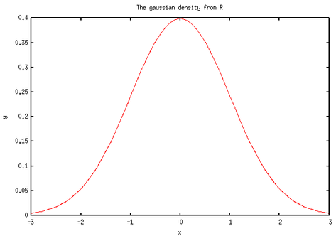
Nothing fabulous actually. But wait, we can do other funny things. First, let’s implement a simplified t-test. There’s already a bunch of handy functions in base/statistics.jl. Basically, we just need to compute a difference of means and a pooled estimate for the variance. Note that we assume equal variance and a two-sided test. I also added a switch-statement for the case of paired samples. This has been tested with the famous Student’s sleep data set (student1908.csv).

function t_test(x, y, paired)
  nx = length(x)
  ny = length(y)
  dobs = mean(y) - mean(x)
  if paired == true && nx == ny
    df = nx - 1
    se = std(x-y) / sqrt(nx)
  else
    df = nx + ny - 2
    se = sqrt(((nx-1) * std(x)^2 + (ny-1) * std(y)^2) / df)
  end
  if paired == false 
    se = se * sqrt(1/nx + 1/ny)
  end
  tobs = dobs / se
  pval = 2*(1 - pt(tobs, df))
  res = HashTable()
  res["stats"] = tobs; res["df"]=df; res["p_value"]=pval
  res
end

dat = dlmread("student1908.csv")
t_test(dat[:,1], dat[:,2], false)  # p = 0.079
t_test(dat[:,1], dat[:,2], true)   # p = 0.003

Nothing really difficult there. Let’s go for a rough PCA, on Fisher-Anderson iris.txt dataset. Julia already has some basic linear algebra functions in base/linalg.jl (plus additional LAPACK bindings in linalg_lapack.jl, including SVD computation):

function scale(x)
  (x - mean(x)) /std(x)
end

function pca(a, standardize)
  if standardize == true
    for i = 1:size(a, 2)
      a[:,i] = scale(a[:,i])
    end
  end
  res = svd(a)
  sd = res[2] / sqrt(size(a, 1) - 1)
  rot = transpose(res[3])
  sd, rot
end

iris = dlmread("iris.txt")
pca(iris[:,1:4], true)

We can also compare results from an SVD and an eigenvalue decomposition:

n = 100
x1 = randn(n)
x2 = randn(n)
x3 = .6 * x1 + randn(n)
X = [x1 x2 x3]
for i = 1:size(X, 2)
  X[:,i] = scale(X[:,i])
end
amap(mean, X, 2)
r = 1/(n-1) * X' * X
res1 = pca(X, false)[1]
res2 = sortr(real(sqrt(eig(r)[1])))

The above code (it probably looks really ugly because these are my very first lines of Julia code!) reminds me of my 4-5 years of Matlab, but overall the documentation points toward interesting features that I just need to learn more.

As a conclusion of this 2-hour session, it is evident that I am missing a lot of things about Julia. There’s a cor method that is supposed to work with one or two vectors, but also with a matrix, but it doesn’t seem to work when I call it like cor(X). I also had some trouble with csv header which when present gave me an Any Array that I know nothing about. Well, in my defense I haven’t finished reading the documentation set, and just started from scratch with a console REPL early in the morning.

A reply by Harlan Harris to a recent question on Cross Validated, Does Julia have any hope of sticking in the statistical community?, summarizes a lot of missing features compared to R. But it still looks like a great project, and it’s always interesting to follow the development of a new programming language from the start.