Consider the problem where there’s no direct solution to $Xb = y$, yet we may be looking for the best approximation of $y$ as a linear combination of the columns of $X$. One of the well-known application of this setting is the linear regression model, of course. Recall that the OLS solution is $\left(X^TX\right)^{-1}X^Ty$.

Rather than inverting the $X$ matrix, we will use QR decomposition, as R does, since we assume a full (column) rank matrix $X$. The QR decomposition reads $X=\underset{m\times n}{Q}\overset{n\times n}{R}$, where $Q^TQ=I_n$ (columns are orthonormal) and $R$ is an upper-triangular invertible matrix. We already discussed this in a previous post. Note that

$$ \left(X^TX\right)^{-1}X^Ty = \left(R^TQ^TQR\right)^{-1}R^TQ^Ty = \left(R^TR\right)^{-1}R^TQ^Ty = R^{-1}Q^Ty. $$

In the end, we only really need to solve $Rx = \bar y$, where $y$ is rotated as $\bar y = Q^Ty$ (in R, this is computed using qr.qty()) and $R$ is triangular, using backward substitution.

More information can be found in this on-line course, which inspired the above notation, and this longer article on the Stan website: The QR Decomposition For Regression Models. For a more detailed treatment, I would suggest Numerical Methods of Statistics (2nd ed.), by John F. Monahan, especially for the connection with Householder transformations (§5.6.).

Let’s implement this approach in Lisp using the magicl package, which provides low-level bindings to BLAS/LAPACK as well as a high-level interface with everything we need for common linear algebra problems (e.g., SVD, Cholesky or QR decomposition, etc.). Other CL libraries are available but this one looks interesting because it is actively maintained by working heroes, including Robert Smith (@stylewarning), who also happens to play piano. As an illustration, here is how one compute the SVD ($U\Sigma V$) of a rectangular matrix:

(defparameter *a* (magicl:from-list '(3.0 2.0  2.0
                                      2.0 3.0 -2.0)
                                    '(2 3)))
(magicl:svd *a*)

This returns the expected results:

$$ \begin{array}{l} U = {\pmatrix {1/\sqrt{2} & 1/\sqrt{2} \cr 1/\sqrt{2} & -1/\sqrt{2}}} \cr \Sigma = {\pmatrix {5 & 0 & 0 \cr 0 & 3 & 0}} \cr V^T = {\pmatrix {1/\sqrt{2} & 1/\sqrt{2} & 0 \cr 1/\sqrt{18} & -1/\sqrt{18} & 4/\sqrt{18} \cr 2/3 & -2/3 & -1/3 }} \end{array} $$

We also need a toy dataset, which will be a subset of one the dataset used by Selvin in his book on S+ (see here for a collection of plots and a recap' of the exercises). Here is a quick glance at the dataset, which describes how birth weight evolves with maternal age for smoking and non-smoking mothers:

Gnuplot script and raw dataset.

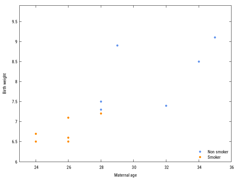
The regression line in the above plot reads $\text{weight} = 3.61 + 0.15\times\text{age} - 0.57\mathbb{I}_{\text{smoking}}$.

Let’s first try to input the data: (be careful, values must be recognized as float, not integers, and of course we need to add a column of one’s for the intercept!)

(ql:quickload :magicl)
(setf *read-default-float-format* 'double-float)
(defparameter *y* (magicl:from-list '(9.1 8.9 8.5 7.4 7.5 7.3 6.7 6.5 7.2 6.5 6.6 7.1) '(12 1)))
(defparameter *X* (magicl:from-list '(1.0 35.0 0.0
                                      1.0 29.0 0.0
                                      1.0 34.0 0.0
                                      1.0 32.0 0.0
                                      1.0 28.0 0.0
                                      1.0 28.0 0.0
                                      1.0 24.0 1.0
                                      1.0 24.0 1.0
                                      1.0 28.0 1.0
                                      1.0 26.0 1.0
                                      1.0 26.0 1.0
                                      1.0 26.0 1.0)
                                    '(12 3)))

The instruction (magicl:qr *X*) should return the two matrices $Q$ and $R$ discussed above. Then, from the expressions above we see that the vector of estimated parameters can be computed as $R^{-1}Q^Ty$, such that we can write:

(multiple-value-bind (Q R)
     (magicl:qr *X*)
   (magicl:@ (magicl:inv R) (magicl:@ (magicl:transpose Q) *y*)))

We get the estimated parameters $(3.606, 0.146, -0.574)$, and $R = {\pmatrix {3.464 & 98.150 & \hphantom{-}1.732 \cr 0.000 & 12.028 & -1.330 \cr 0.000 & 0.000 & \hphantom{-}1.109}}$.

Well, that’s a bit convoluted but that worked. Next time, we’ll see how the GSLL can be used to solve similar problems.