Wolfram, né Mathematica, 14.3 introduced a cool new feature for graphical exploratory data analysis: loess fitting. It is already discussed at length on Stephen Wolfram’s blog post about this last release, but I was interested in trying it myself. Needless to say I don’t do much applied statistical work these days. I miss compitational statistics a lot and I expect to come back to it at some point, though.

Without further ado, let’s consider data analyzed in this old course of mine, specifically the FEV dataset. It is available in R format, which is well managed by the omnibus Import function:

data = Import["fev.rds", "Dataset"]
data[1;;5, All]

We are interested in describing the relationship between the FEV (fev) and age (age) in male and female (sex). Here is a basic scatterplot:

data[ListPlot, {"age", "fev"}]

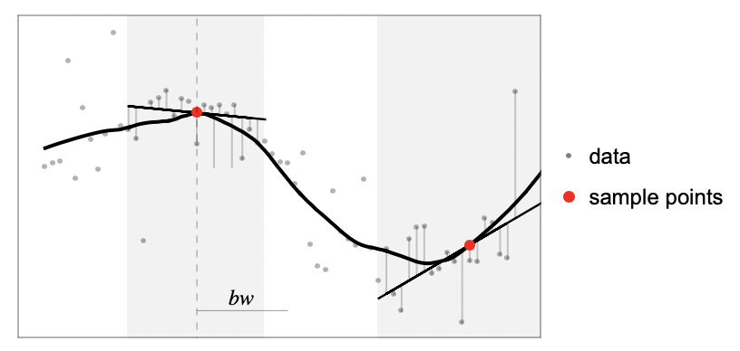
The Wolfram help center does a good job at explaining what is LOESS smoothing. Here we are interested in small departure from the linearity assumption in usual OLS.

There are various ways to displays a scatterplot smoother. First, we can just fit a local smoother:

LocalModelFit[ToTabular[data[All, {"age", "fev"}]]]

We use the tabular data structure introduced in version 14.2. It returns a FittedModel, like other statistical models in Wolfram (e.g., LinearModelFit), although there’s no best fitting model such that we cannot use Normal (despite what the online help says about the “BestFit” slot), We can obtained the predicted (interpolated) values using the “PredictedResponse” slot.

Here is another way to perform the same task: we can directly ask for a plot using ListPlot[data[All, {"age", "fev"}], PlotFit -> "Local"]. We could also work directly with a list of pairwise values, instead of association lists:

trend = LocalModelFit[List @@@ Normal[data[All, {"age", "fev"}]]];
Show[ListPlot[data[All, {"age", "fev"}]],
 Plot[trend[x], {x, 4, 18}, PlotRange -> All, PlotStyle -> Red],
 PlotRange -> All]

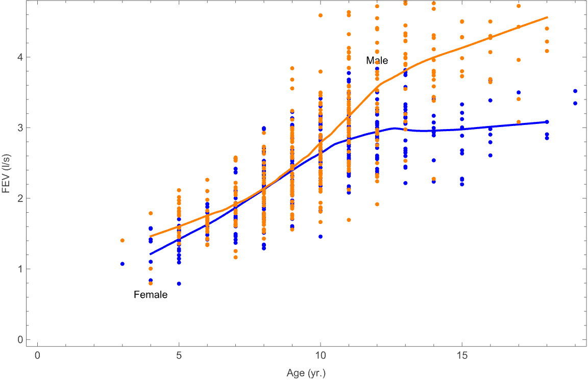
Finally, we can fit a separate loess curve for male and female using GroupBy on the structured dataset:

g = GroupBy[data[All, {"age", "fev", "sex"}], "sex"][[All, All, 1 ;; 2]];
male = LocalModelFit[List @@@ Normal[g[[1]]]];
female = LocalModelFit[List @@@ Normal[g[[2]]]];
Show[ListPlot[g[[1]], PlotStyle -> Blue,
  PlotLabels -> Placed["Male", Above]],
 Plot[male[x], {x, 4, 18}, PlotStyle -> Blue],
 ListPlot[g[[2]], PlotStyle -> Orange,
  PlotLabels -> Placed["Female", Below]],
 Plot[female[x], {x, 4, 18}, PlotStyle -> Orange], Frame -> True,
 ImageSize -> Large, FrameLabel -> {"Age (yr.)", "FEV (l/s)"}]

Of course, we could also play with the bandwidth parameter, as illustrated in this example on Stack Exchange.