In an older post I showed how we could fit a Logistic regression using Racket builtin linear algebra routines.

It is not difficult to import a CSV file and get a working Table for a Logistic regression model, or any other model from the Exponential family really. Here’s how I did for the classical low birth weight dataset from Hosmer & Lemeshow¹, where I consider a single predictor (age of the mother):²

data = Import["~/Documents/work/tutors/CESAM/cours/Stata/birthwt2.csv"];
dt = data[[2 ;;, {2, 1}]];
m = GeneralizedLinearModelFit[dt, x, x, ExponentialFamily -> "Binomial"];

Note that we could also use SemanticImport to get a “Dataset” structured array, but since it is not callable from GeneralizedLinearModelFit, let’s stay with classical list of lists. From here now, almost all we need is now available in our “FittedModel” m, and we can even display the regression equation using the following incantation:

m // Normal

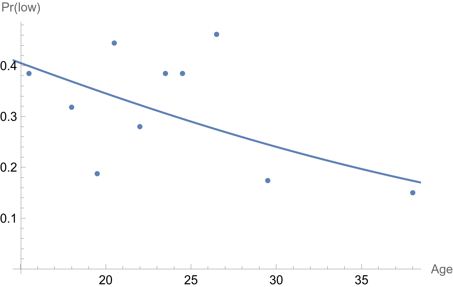
Now, what I really want is to display the logistic fitted curve together with observed proportions of low birth weights (< 2.5 kg) at each decile of age (see my other post to get an idea of this observed vs. fitted proportion display). In Mathematica, there are some grouping and binning functions (AggregatedEntityClass, SplitBy, GatherBy, BinLists, BinCounts) or one could also rely on histogram binning.

First we need to add a column indicating to which decile each value of age belongs to. Here is my solution, which relies on the empirical distribution function instead of the Quantile function. This is partly inspired by a solution proposed by Sjoerd C. de Vries to a similar problem:

ecdf = EmpiricalDistribution[dt[[All, 1]]];
f[x_] := 1 + CDF[ecdf, x] 10 // Floor
qvalues = Map[f, dt[[All, 1]]];
qvalues = qvalues /. {11 -> 10}; (* FIXME: account for max value *)

Here, an instruction like MapThread[Append, {dt, qvalues}] will simply append a new column holding the decile index for each row. We would like, however, to replace each decile index with the corresponding class center from the real values, which can be computed as follows:

tens = Quantile[dt[[All, 1]], Range[0, 1, .1]];
centers = Total[{Most[tens], Differences[tens]/2}];

Then, we need a replacement rule to tell Mathematica how to perform the desired mapping:

SetAttributes[g, Listable]
g[a_, b_] := a -> b

Finally, we will add a new column to our data set to reflect class membership for each observation, and plot both the prediction and the mean observed frequencies for each decile:

dt = MapThread[Append, {dt, qvalues /. g[Table[x, {x, 10}], centers]}]
obs = GroupBy[Sort[dt[[All, 2 ;;]]], Last -> First, Mean]
Show[ListPlot[obs], Plot[m[x], {x, 14, 45}], AxesLabel -> {"Age", "Pr(low)"}]