Here is a little post about using Mathematica to study basic model of DNA substitutions, including the Jukes-Cantor model, and more generally likelihood-based phylogenetic tree inference.

Warming up

Say we are interested in comparing the genome of two species, assuming they have a common ancestor, which should be the case, at least for eukaryotes. For various reasons, DNA substitutions occur over time on the genome and the two species may look different at a certain point in time when comparing the pairwise alignment of their sequences. However, not all substitutions are equally likely and, for example, we may assume the following transition matrix, $Q$, which I took from this nice tutorial (PDF):

$$ \begin{pmatrix} -0.886 & 0.190 & 0.633 & 0.063\cr 0.253 & -0.696 & 0.127 & 0.316\cr 1.266 & 0.190 & -1.519 & 0.063\cr 0.253 & 0.949 & 0.127 & -1.329 \end{pmatrix} $$

where the rows and columns denote the nucleotide A, C, G and T. Hence, if we are in state A, we will wait an exponetial amount of time, with parameter $-q_{ii}=0.886$. The probability to observe the transition A→C is then $-q_{ij}/q_{ii}=\tfrac{0.190}{0.886}$.

Now, let’s consider that events occur over time, $t$, with rate $\lambda$. The waiting time before observing the next event is then described by an exponential distribution, $f(t)=\lambda e^{-\lambda t}$, while the waiting time for observing the $k$-th event follows a Gamma distribution, $f(t)=\frac{\lambda^k}{\Gamma(k)}t^{k-1}e^{-\lambda t}$, using shape-rate parametrization. Note that since $k$ is necessarily an integer, $\Gamma(k)=(k-1)!$. Finally, the number of events that may occur in the interval $T$ follows a Poisson distribution with parameter $\lambda T$, that is $\Pr(k) = \frac{e^{-\lambda t}(\lambda T)^k}{k!}$.

So, if we start in state A, we will have to wait $\exp(0.886)=2.425$ units of time, and the probability to switch to another state are 0.214 (for C), 0.714 (G) and 0.071 (T). The most likely switch, A→G, implies that we will then have to wait $\exp(-0.633)=0.531$ unit of time. And so on… For each starting state, it is easy to compute the frequencies of ending states over the whole study time $t$, which we will call the “divergence time”.

Here is a quick illustration using Mathematica:

Q = {{-0.886, 0.190, 0.633, 0.063}, {0.253, -0.696, 0.127,
    0.316}, {1.266, 0.190, -1.519, 0.063 }, {0.253, 0.949,
    0.127, -1.329}};
Total[Q, {2}]

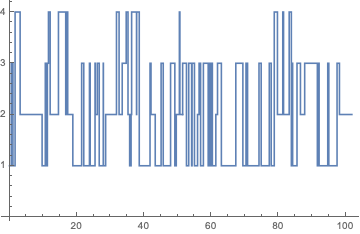
Note that I checked that the rows (or the “columns” in Mathematica parlance) sum to zero indeed. Even if Mathematica offers to correct for non-zero sum rows, it’s better to check beforehand. I got {0., 5.55112*10^-17, 0., 0.}, which looks fine. Below, I define a continuous Markov random process and draw a sample of data using 100 iterations, assuming the initial state is A:

p = ContinuousMarkovProcess[{1, 0, 0, 0}, Q];
data = RandomFunction[p, {0, 100}];
ListStepPlot[data]

PDF[p[\[Infinity]], 2]

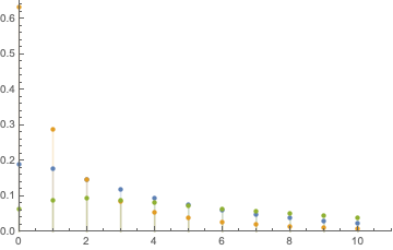
According to our manual estimation, after the first iteration we will most likely end up in state 3 (G). We can ask Mathematica what is the distribution of the number of steps required for the process to pass from the initial state (A) to any other state for the first time:

Table[PDF[FirstPassageTimeDistribution[p, j], k], {j, {2, 3, 4}}];
DiscretePlot[Evaluate[%], {k, 0, 10}, PlotRange -> {{0, 11}, {0, 0.7}},
  PlotLegends -> {"C", "G", "T"}]

Finally, the limiting transition matrix is obtained using MarkovProcessProperties[p, "LimitTransitionMatrix"], and we are in close agreement with the results printed in the tutorial:

$$ \begin{pmatrix} 0.400149 & 0.299915 & 0.200167 & 0.099769\cr 0.400149 & 0.299915 & 0.200167 & 0.099769\cr 0.400149 & 0.299915 & 0.200167 & 0.099769\cr 0.400149 & 0.299915 & 0.200167 & 0.099769 \end{pmatrix} $$

The Jukes-Cantor model

Let’s now consider a simpler model. A tutorial is available on Jay Taylor website. According to the Jukes-Cantor model (Jukes, T. H. and Cantor, C. R., Evolution of protein molecules. In Mammalian Protein Metabolism, ed. Munro, H. N., pp. 21-132, New York: Academic Press, 1969), the rate matrix reads:

$$ \begin{pmatrix} -3\mu & \mu & \mu & \mu\cr \mu & -3\mu & \mu & \mu\cr \mu & \mu &-3\mu & \mu\cr \mu & \mu & \mu & -3\mu \end{pmatrix} $$

This means that each nucleotide have a constant rate of mutation $\mu$. The probability that both species have the same nucleotide on an homologous site equals $\Pr(\text{same}) = \frac{1}{4}(1+3e^{-8\mu t})$, hence $\Pr(\text{different}) = 1 - \Pr(\text{same}) = \frac{3}{4}(1-e^{-8\mu t})$. Notice that the total time elapsed along the genealogy is $2t$. Now, if we compare $m$ sites, on which there are $n$ (independent) substitutions and we write $x = -8\mu t$, then the likelihood for the divergence time can be written:

$$\ell(t;n) = \left(\frac{1+3e^x)}{4}\right)^{m-n}\left(\frac{3(1-e^x)}{4}\right)^n.$$

The log-likelihood is then

$$\mathcal{L}(t;n) = (m-n)\log(1+3e^x) + n\log(1-e^x) + \text{some constant} \perp\hskip-5pt\perp t.$$

The MLE for the divergence time is obtained by differentiating $\mathcal{L}(t;n)$ wrt. $t$ and finding its root. This yields the following equation:

$$(m-n)\frac{-24e^x}{1+3e^x} + n\frac{8e^x}{1-e^x} = 0.$$

Mathematica gives me the solution 1 - (4 d)/(3 L) for $x$:

Solve[d (8 x)/(1 - x) + (L - d) (-24 x)/(1 + 3 x) == 0, x]
Simplify[%]

Solving for $t$ since we set $x = -8\mu t$, we get the estimate for the divergence time $\hat t = -\frac{1}{8\mu}\log\left(1-\frac{4n}{3m}\right)$.

Here is how I setup the basic parameters for simulating data obeying the Jukes and Cantor model:

bases = {"a", "c", "g", "t"};
exon = {.25, .25, .25, .25};
α = 0.001;
n = 100;
s = RandomChoice[exon -> bases, n];
Q = {{1 - α, α/3, α/3, α/3}, {α/3, 1 - α, α/3, α/3}, {α/3, α/3,
  1 - α, α/3}, {α/3, α/3, α/3, 1 - α}};

Note that it is important to not use MatrixForm at this step, otherwise we will get in trouble with matrix multiplication later. The rate is controlled by $\alpha$ and s is a random sequence of nucleotides. The distribution of nucleotide frequencies is close to the expected ones (1/4), and multiplying the transition matrix Q by the vector of observed frequencies fb yields an updated vector of frequencies. Here I got {0.230027, 0.25, 0.27996, 0.240013}:

fb = N[Tally[s][[All, 2]]/n, 6]
Q.fb

We can repeat the same process, say 10 times using Nest, and also display how the frequency of state A evolves over 10,000 iterations:

Nest[Function[x, Q.x], fb, 10]
ListPlot[NestList[Function[x, Q.x], fb, 10000][[All, 1]],
  PlotRange -> {{0, 10000}, {0.23, 0.27}}]

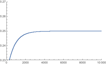
This is in agreement with the model specifications and $\Pr(A)=\frac{1}{4}$.