Measures of accuracy for classification
I just discovered a not so recent article providing an overview of measures of accuracy in predictive classification tasks. Specifically, this article focuses on the pros and cons of different measures of classification accuracy with a particular emphasis on percentage-, distance-, correlation-, and information-based indices for binary outcomes: Baldi, P., Brunak, S., Chauvin, Y., Andersen, C.A.F., and Nielsen, H., Assessing the accuracy of prediction algorithms for classification: an overview, Bioinformatics (2000) 16(5): 412-424.
Here is the abstract:
We provide a unified overview of methods that currently are widely used to assess the accuracy of prediction algorithms, from raw percentages, quadratic error measures and other distances, and correlation coefficients, and to information theoretic measures such as relative entropy and mutual information. We briefly discuss the advantages and disadvantages of each approach. For classification tasks, we derive new learning algorithms for the design of prediction systems by directly optimising the correlation coefficient. We observe and prove several results relating sensitivity and specificity of optimal systems. While the principles are general, we illustrate the applicability on specific problems such as protein secondary structure and signal peptide prediction.
Let’s start by considering a two-way table looking like the one shown below
| M+ | M- | |
| D+ | TP | FN |
| D- | FP | TN |
where M and D are predicted and true class membership (+/- means positive/negative instances in both cases). The corresponding cells sum to 1 and read as
- TP (resp. TN) for true positive (resp. negative), the number of times a positive (resp.negative) instance is correctly classified;
- FP (resp. FN) for false positive (resp. negative), the number of time a positive (resp.negative) instance is incorrectly classified.
The task is to derive a suitable way to summarize performance accuracy of a given classification algorithm based on these four numbers, which amounts to define a certain distance between M and D.
Percentage-based measures
The percentages of correct positive (PCP) and negative (PCN) predictions are known as the sensitivity and specificity; they are given by
$$ \text{PCP}=\frac{\text{TP}}{\text{TP}+\text{FN}},\quad \text{PCN}=\frac{\text{TN}}{\text{TN}+\text{FP}}. $$
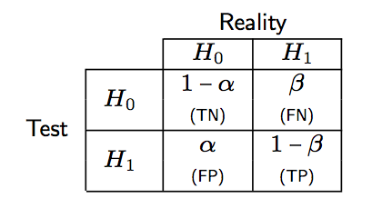
Of note, we have PCP = Pr(instance classified as positive | instance is truly positive), whereas in a statistical decision framework, the Type I error risk is α = Pr(instance classified as positive | instance is truly negative). The following Table summarizes the correspondence between decision theory and classification results.

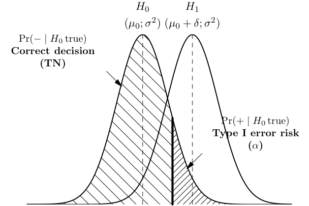
As shown below, a correct rejection of H0 occurs with probability 1 − α and may be considered as test specificity.

Distance-based measures
Any Lp distance between M and D, defined as
$$ L^p=\left(\sum_i |d_i-m_i|^p \right)^{1/p}, $$
can be used, but usually these are the L1 (Hamming), L2 (Euclidean), or L∞ (sup). In the binary case, the Lp distance reduces to (FN+FP)1/p. For the Hamming distance, it is worth noting that it is simply FP+FN, so that it is equivalent to a percentage measure. However, as it does not account for possible imbalance between positive vs. negative instances, it becomes poorly useful when this ratio moves away from 50:50. Also, in the binary case, the euclidean distance reduces to the Hamming distance.
Correlation-based measures
Let’s recall the classical Pearson’s correlation coefficient:
$$ C=\sum_i\frac{(d_i-\bar d)(m_i-\bar m)}{\sigma_D\sigma_M}. $$
I learned that, for binary variables, it is also known as Matthews correlation coefficient, although it is also known as the Phi coefficient in the psychometric literature. Using vector notation, we have
$$ \begin{align} C &= \frac{(\mathbf D-\bar d\mathbf 1)(\mathbf M-\bar m\mathbf 1)}{\sqrt{(\mathbf D-\bar d\mathbf 1)^2}\sqrt{(\mathbf M-\bar m\mathbf 1)^2}} \ &= \frac{\mathbf{DM}-N\bar d\bar m}{\sqrt{(\mathbf D^2-N\bar d^2)(\mathbf M^2-N\bar m^2)}} \end{align} $$
where 1 denotes an N-dimensional unit vector. By writing C as in the above expression, we see immediately that if D and M are normalized, then the L2 distance
$$ (\mathbf D - \mathbf M)^2=2-2\mathbf{DM}=2-2C. $$
Moreover, when dealing with binary variables, we have D2=TP+FN, M2=TP+FP, and DM=TP. Finally, the preceding equation can be written
$$ C=\frac{\text{TP}-N\bar d\bar m}{N\sqrt{\bar d\bar m(1-\bar d)(1-\bar m)}}. $$
And since d̄=(TP+FN)/N, and m̄=(TP+FP)/2, we finally have
$$ C=\frac{\text{TP}\times\text{TN}-\text{FP}\times\text{FN}}{\sqrt{(\text{TP}+\text{FN})(\text{TP}+\text{FP})(\text{TN}+\text{FP})(\text{TN}+\text{FN})}}. $$
As for other interesting references, I would suggest the following articles:
- Ambroise, C and McLachlan, GJ. Selection bias in gene extraction on the basis of microarray gene-expression data, PNAS (2002) 99(10): 6562-6566.
- Saeys, Y, Inza, I, and Larrañaga, P. A review of feature selection techniques in bioinformatics, Bioinformatics (2007) 23(19): 2507-2517.
- Dougherty, ER, Hua J, and Sima, C. Performance of Feature Selection Methods, Current Genomics (2009) 10(6): 365–374.