Lately, I started taking some notes on Next Generation Sequence analysis, more specifically RNA-Seq data. Most of my textbooks are currently outdated, especially the one on Bioconductor: Bioinformatics and Computational Biology Solutions Using R and Bioconductor, by Gentleman and coll. The last time I was doing genomic statistics was in 2009-2010 and NGS was just becoming the new way of analysis big data in biology.

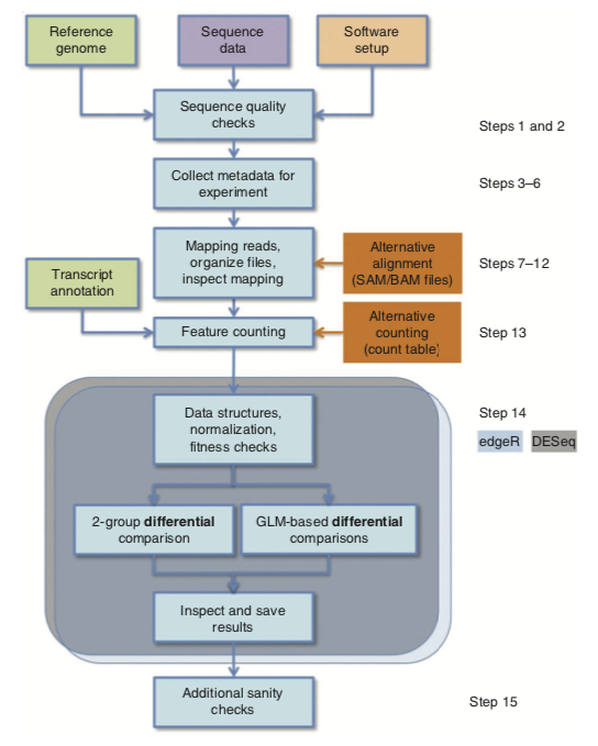
All in one, RNA-Seq consists in a series of extraction, preprocessing and statistical analysis, namely: DNA extraction from a sample, DNA sequencing, Alignment of sequencing reads to a reference genome, Basic exploratory data analysis, Identification of genomic variants (SNPs, small insertions and deletions), Gene quantification (i.e., statistics on count data). But see the following picture which highlights a typical workflow using R :¹

In what follows, I will review two tools that are quite handy if you want things done in a resonnable amount of time. This is does not mean that this the perfect solution — there are far better accurate workflow for data preprocessing — but this may help perform batch analysis in case you have large amount of data and seek an efficient way for screening of candidate gene sets, for instance. I will be using data available on the JGI website, and other data that I cannot share here so that I won’t reproduce R outputs. I hope, however, that the following R code is enough to help you get started with your own dataset.

Data preprocessing

It is beyond the scope of this short note to review all the different software that can be used to perform alignment of reads on a reference genome. Let us say that TopHat2 is probably the best when it comes to findind splice junctions. However, it is also possible to use pseudo-alignment with kallisto, and it is much (much) faster. If reads are in SRA format, they will need to be converted to Fastq files using the sratoolkit.

A sample shell script is provided below:

#!/usr/bin/env bash

PREPROCESS=1

if [ $PREPROCESS -eq 1 ]
then
    ## SRA -> Fasta (parallel runs)
    for file in *.sra
    do
        fastq-dump "${file}"  &
    done

    ## Build index of genome
    kallisto index -i Podans1_GeneCatalog_transcripts_20171002.nt.idx \
        Podans1_GeneCatalog_transcripts_20171002.nt.fasta
fi

## Quantification
for file in *.fastq
do
    kallisto quant -i Podans1_GeneCatalog_transcripts_20171002.nt.idx \
        -o out."${file%.*}" \
        --single -l 100 -s 5 -b 20 --seed 101 --threads=4 "${file}"
        # --pseudobam
done

Once the data files have been processed, we should have a series of abundance data, counts and TPM values.²

Differential analysis

Basically, NGS analyses (RNA, CHIP, etc.) need to account for within-group variance estimates when analysing lot of genes, hence the need to pool information across genes. The DESeq approach detects and corrects dispersion estimates that are too low through modeling of the dependence of the dispersion on the average expression strength over all samples. In addition, it provides a novel method for gene ranking and the visualization of stable estimates of effect sizes.³ The deseq2 package further includes shrunken fold changes (with SE).

We need two data frames before running the statistical analysis: a table of counts (or TPM values from kallisto or salmon), and a table describing the experimental condition. Note that each run must come with at least two replicates (ideally, three). Here are the basic steps to import counts data and setup the design matrix:

library("DESeq2")
library("tximport")
datadir <- dir(".", pattern = "out.\\.*")
files <- file.path(datadir, "abundance.h5")
names(files) <- gsub("out.", "", datadir)
samples <- data.frame(run = names(files), condition = c("4h", "48h", "24h"))
txi <- tximport(files, "kallisto", txOut = TRUE)
dds <- DESeqDataSetFromTximport(txi, colData = samples, design = ~ condition)

Two preprocessing stages are worth considering before dwelling into gene quantification per se: quality control and normalization. Quality control amounts to controlling the number of genes having non-zero counts in all samples. If this number is very low, it is likely that something went wrong, at least with some of the samples. Based on the DESeq table of counts, we can proceed as follows in R:

gene_counts <- counts(dds)
counts_per_sample <- apply(gene_counts, 1, function(x) all(x) > 0)
cat(sum(counts_per_sample), "out of", nrow(dds), "\n")

Normalization refers to the comparison of size factors defined as the median of ratios of each sample to a virtual reference sample (median of each gene’s values across samples). Those ratios are expected to match the ratios of the library sizes and be roughly equal to one. Dividing each column of the count table by the corresponding size factor yields normalized count values, which can be scaled to give a counts per million interpretation. Note that this is different from the approach taken by edgeR, which considers the trimmed mean of M values. An MA plot can be used to show the average vs. mean–difference of log fold change, centered around 0, and it is expected to observe higher variability of log ratios at lower counts.

A PCA or simple heatmap of the results of hierarchical clustering of the sample data can be used to assess overall similarity between samples. We expect triplicate to cluster together while samples from very different experimental conditions are expected to be far away one from the other. Of note, it is useful to apply a regularized log–transformation on the raw counts to avoid the impact of few highly variale genes, hence considering a roughly equal contribution from all genes. For genes with high counts, this mostly resembles a log2 transformation, whereas for genes with low counts, this shrunkens values toward gene’s average across amples. It is important to note that this is only for exploratory analysis; for statistical modeling, raw counts should be preferred since DESeq will handle appropriate correction automagically:

rld <- rlogTransformation(dds, blind = TRUE)
dd <- as.matrix(dist(t(assay(rld))))
library(pheatmap)
pheatmap(dd)
plotPCA(rld, intgroup = c("condition"))

The statistical model underlying differential analysis of count data is a Negative Binomial, which contrary to the standard Poisson model allows to account for overdispersion (i.e., variance greater than mean). Variance is modeled as $\mathbb{V}[NB(\mu, \alpha)]=\mu+\alpha\mu^2$, and the very first step in differential analysis is to get an estimate of the dispersion parameter for each gene (independent of the condition, which is sensible since there is usually a low number of replicates). Notice that for genes with very low read counts, the large amount of Poisson noise prevent those genes from exhibiting any DE at all, and DESeq performs independent filtering automatically to discard such low signals and to increase statistical power for the remaining gene candidates. The asymptotic dispersion for highly expressed genes can be seen as a measurement of biological variability in the sense of a squared coefficient of variation: a dispersion value of 0.01 means that the gene’s expression tends to differ by typically $\sqrt{0.01}=10%$ between samples of the same treatment group. The R procedure estimateDispersions allows to compute (and visualize) dispersion estimates as a function of mean normalized counts.

The statistical test used to assess whether genes are differentially expressed between samples is a Wald test (nbinomWaldTest), with FDR correction for multiple testing. Benjamini–Hochberg’s adjusted p-values can then be ranked to highlight the top genes. Usually, the statistical threshold is set at 0.1, and not 0.05 as in standard null hypothesis statistical testing.

ddstab <- estimateDispersions(estimateSizeFactors(dds))
r <- results(nbinomWaldTest(ddstab), pAdjustMethod = "BH")
table(r$padj < 0.1)
## r@metadata$filterThreshold

The inspection of the distribution of (unadjusted) p-values is helpful to verify that the null distribution for the test statistic is viable. If the histogram does not exhibit an uniform pattern (e.g., U or hill shape), then it is likely that the $\mathcal{N}(0,1)$ null distribution is not appropriate. See the fdrtool and locfdr packages for further strategies about controlling global or local FDR, and empirical null modeling allowing to estimate the variance of the null model (expected to be 1, per the $\mathcal{N}(0,1)$ hypothesis).

Once the model is fitted, it is possible to extract the top genes using, e.g.:

plotMA(r)
names(dds)[which(r$padj < 0.1)]

Then, it is harder time where you will have to make sense of all oh those results using Gene Ontology and the like.