Paired preference models
Much of this discussion is supported by Agresti’s book, Categorical Data Analysis (Wiley, 2002), and the overwhelming work of Laura Thompson who adapted the analysis with S-PLUS and R. However, some methods are rather specific of Psychometrics like the Facets Model presented in the first section.
The psychometrician’s way: Thurstone Model and the Partial Credit Model
Here, we shall focus on a more or less sophisticated way of assessing observers’ preference in a ranking task, gathered from an article published by Tom Bramley in the Journal of Applied Measurement (2005, strong6(2)/strong: 202–223): A Rank-Ordering Method for Equating Tests by Experts Judgment. According to Thurstone’s paired comparisons model(1), but see also Wikipedia, “pairs of object are compared with respect to a single attribute which is conceived as being represented in the judge’s mind as a psychological latent trait.” Following Bramley’s notation, this is modeled as
$$ \ln \left[\frac{P_{ij}}{1-P_{ij}}\right] = B_i - B_j, $$
where $B_i$ and $B_j$ correspond to measures recorded for item $i$ and $j$, respectively. $P_{ij}$ can be conceived as the probability that item $i$ “beats” (i.e., is being ranked above than) item $j$ for any observer (it’s just an odds). In contrast, with the Partial Credit Model (PCM), the model fitted is
$$ \ln\left[P_{irk}/(1-P_{ir(k+1)})\right] = B_i - D_{rk}. $$
Now, the model becomes an adjacent-category model where $B_i$ is the measure for item $i$ and $D_{rk}$ is the difficulty of scale category $k$ relative to category $k+1$ in ranking $r$.
The Bradley-Terry Model for paired preferences
If we consider a square table whose $K$ entries refer to the number of times category $a$ is preferred to category $b$, after emptying the main diagonal, the B-T Model can be expressed as
$$ \log\frac{\Pi_{ab}}{\Pi_{ba}} = \beta_a - \beta_b, $$
where
$$ \Pi_{ab} = \frac{\exp(\beta_a)}{\exp(\beta_a)-\exp(\beta_b)}, $$
is the probability that $a$ is preferred to $b$. It can be shown that the number $n_{ab}$ (people who prefer $a$ compared to $b$) follows a binomial distribution whose parameter is the above estimated probability.
The R package BradleyTerry includes the necessary code to carry out the test of such model. D. Firth also wrote an article in the Journal of Statistical Software (2005, 12(1)), Bradley-Terry Models in R. As an example, let’s consider the data on baseball season in the Eastern Division (Agresti, 2nd edition, p. 437) which are summarized in the following table. Values in parentheses represent SAS fit of B-T model.
| Winning Team | Milwaukee | Detroit | Toronto | New York | Boston | Cleveland | Baltimore |
| Milwaukee | — | 7 (7.0) | 9 (7.4) | 7 (7.6) | 7 (8.0) | 9 (9.2) | 11 (10.8) |
| Detroit | 6 (6.0) | — | 7 (7.0) | 5 (7.1) | 11 (7.6) | 9 (8.8) | 9 (10.5) |
| Toronto | 4 (5.6) | 6 (6.0) | — | 7 (6.7) | 7 (7.1) | 8 (8.4) | 12 (10.2) |
| New York | 6 (5.4) | 8 (5.9) | 6 (6.3) | — | 6 (7.0) | 7 (8.3) | 10 (10.1) |
| Boston | 6 (5.0) | 2 (5.4) | 6 (5.9) | 7 (6.0) | — | 7 (7.9) | 12 (9.8) |
| Cleveland | 4 (3.8) | 4 (4.2) | 5 (4.6) | 6 (4.7) | 6 (5.1) | — | 6 (8.6) |
| Baltimore | 2 (2.2) | 4 (2.5) | 1 (2.8) | 3 (2.9) | 1 (3.2) | 7 (4.4) | — |
The data can be downloaded from here: baseball1987.dat.
If we look at the result of the BT fit, we see that…
baseball <- read.csv("baseball1987.dat", na.strings=".")
library(BradleyTerry)
bb.BT <- BTm(baseball ~ ..)
The results match those displayed in Table 10.11 of Agresti’s book, where model estimates of $\beta_a$ (setting $\beta_7 = 0$, for Baltimore) and $\exp(\beta_a)$ (with the constraint $\sum_a \exp(\beta_a) = 1$).
Coefficients:
            Estimate Std. Error z value Pr(>|z|)
..Boston      1.1077     0.3339   3.318 0.000908 *
..Cleveland   0.6839     0.3319   2.061 0.039345 *
..Detroit     1.4364     0.3396   4.230 2.34e-05 *
..Milwaukee   1.5814     0.3433   4.607 4.09e-06 *
..New.York    1.2476     0.3359   3.715 0.000203 *
..Toronto     1.2945     0.3367   3.845 0.000121 *
Here, we see that the estimated probability that Boston won against New York is
$$ \Pi_{15}=\exp(\beta_1)/\big[\exp(\beta_1)+\exp(\beta_5)\big]=0.46, $$
or
exp(coef(bb.BT))["..Boston"] / (exp(coef(bb.BT))["..Boston"] +
  exp(coef(bb.BT))["..New.York"])
As proposed by L. Thompson, it is also possible to fit the B-T model using GLM and auxiliary variables, e.g.
bb.BT2 <- glm(Freq ~ 1 + Milwaukee + Detroit + Toronto +
              NY + Boston + Cleveland, family=binomial)
summary(bb.BT2)
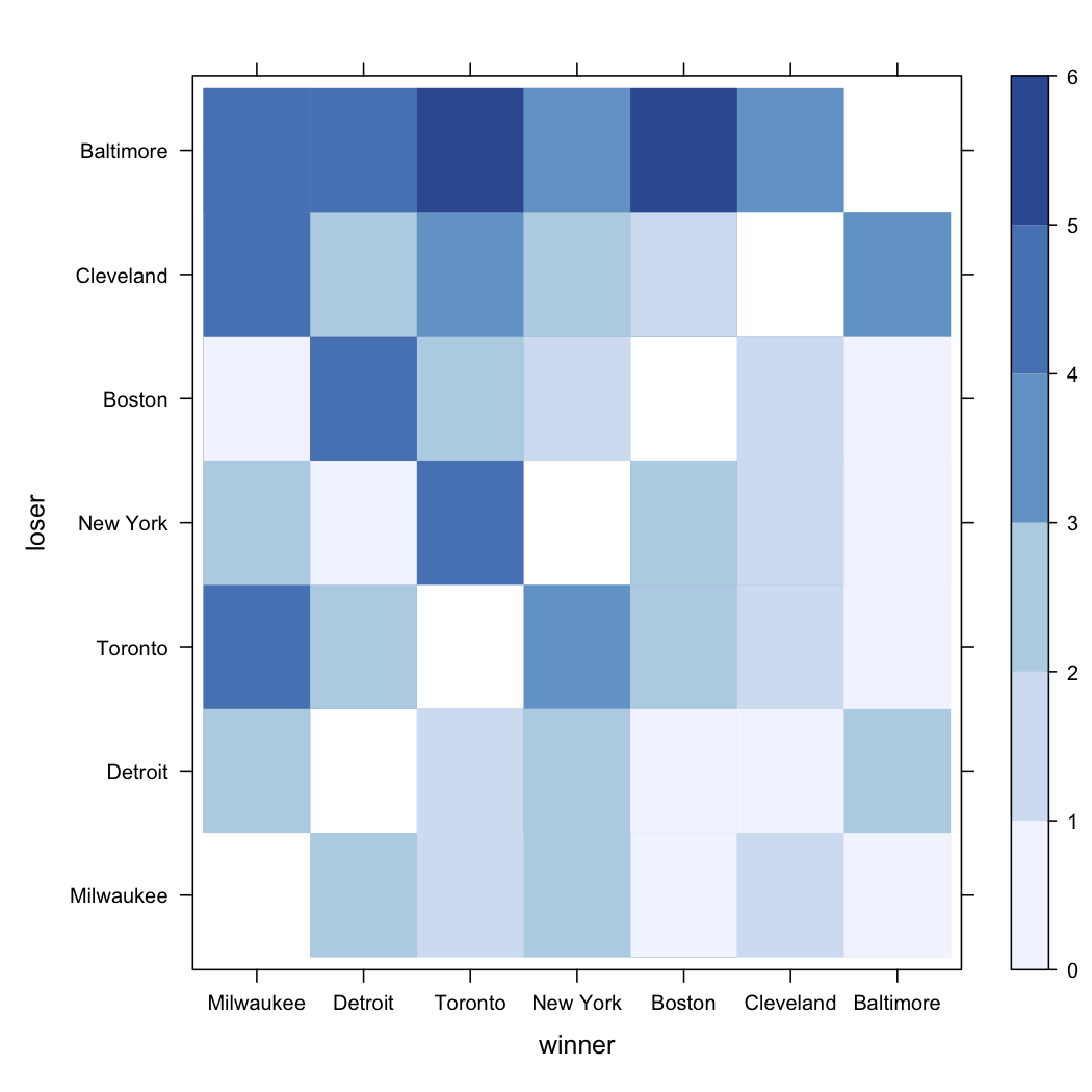
Finally, we might represent the data using a matrix-like representation, where each cell reflect the actual frequency of wins, as suggested below. A more interesting plot would be to show the estimated probability, which is left as an exercise to the reader.
library(lattice)
library(RColorBrewer)
levelplot(Freq~winner+loser, baseball,
          col.regions=brewer.pal(7,"Blues"), at=0:6)

References
- Thurstone, L.L. (1927). A law of comparative judgment. Psychological Review, 3, 273-286.
- Andrich, D. (1978). Relationships between the Thurstone and Rasch approaches to item scaling. Applied Psychological Measurement, 2(3), 451-462.
- Luce, R.D. (1997). Quantification and symmetry: Commentary on Michell, Quantitative science and the definition of measurement in psychology. British Journal of Psychology, 88, 395-398.
- Bradley, R.A. and Terry, M.E. (1952). Rank analysis of incomplete block designs I: The methods of paired comparisons. Biometrika, 39, 324-345.
- Husson, F. and Causeur, D. (2004). Une extension bidimensionnelle du modèle de Bradley-Terry pour les comparaisons par paires. XXXVièmes journées de Statistique, Montpellier, 24-28 mai 2004.
- Conner, G.R. and Grant, C.P. (2000). An extension of Zermelo’s model for ranking by paired comparisons. European Journal of Applied Mathematics, 11, 227-245.