PCA by hand

September 10, 2026

Usually, statistical software implements principal component analysis (PCA) using eigen decomposition, based on the correlation or covariance matrix, or singular value decomposition (SVD), based on the rectangular dataset.

Consider the Holzinger & Swineford dataset from the lavaan R package. It is composed of responses given by 301 children to a battery of subtests assessing various abilities like spatial, treatment speed or verbal abilities. This is usually a good candidate dataset for a second-order factor model, but let’s stick to a standard PCA on the visual dimension.

Here’s how I would perform a PCA using Stata builtin features: (dataset in CSV format)

import delimited "hs.csv"
rename (x1-x3) (visual cubes paper)
pca visual-paper

We get the following eigenvalues and eigenvectors (Comp1 and Comp2 for the first two components):

Principal components/correlation                 Number of obs    =        301
                                                 Number of comp.  =          3
                                                 Trace            =          3
    Rotation: (unrotated = principal)            Rho              =     1.0000

    --------------------------------------------------------------------------
       Component |   Eigenvalue   Difference         Proportion   Cumulative
    -------------+------------------------------------------------------------
           Comp1 |       1.7221      .999352             0.5740       0.5740
           Comp2 |      .722752       .16761             0.2409       0.8150
           Comp3 |      .555143            .             0.1850       1.0000
    --------------------------------------------------------------------------

Principal components (eigenvectors)

    ----------------------------------------------------------
        Variable |    Comp1     Comp2     Comp3 | Unexplained
    -------------+------------------------------+-------------
          visual |   0.5900   -0.4802    0.6491 |           0
           cubes |   0.5297    0.8369    0.1377 |           0
           paper |   0.6093   -0.2626   -0.7482 |           0
    ----------------------------------------------------------

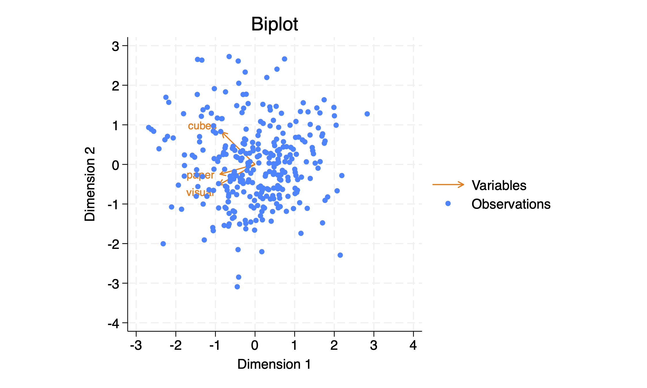
Post-estimation graphical procedures allows to project both the variables and the individuals in the factorial space using Gabriel PCA biplot which provides a good approximation of the Mahalanobis distance between observations.¹

Now, let’s do it by hand using Mata:

mata
X = st_data(., ("visual", "cubes", "paper"))
n = rows(X)
Xc = (X :- mean(X)) :/ diagonal(sqrt(variance(X)))'
U = s = Vt = .
svd(Xc, U, s, Vt)
(s :^ 2) / (n - 1)
Vt'
end

Et voilà ! The only trick is to standardize the raw matrix, so that we get scaled eigenvectors (Vt). Mata is not that hard and you want to be a serious programmer, right?

♪ Lene Lovich • I Think We’re Alone Now

The ggbiplot R package, by Michael Friendly, offers the same projection. It’s funny the original version of ggbiplot was developed by Vince Vu to answer a question on Cross Validated. Good ol’ times. ↩︎

aliquote.org

PCA by hand

See Also