Recently, I was reading some posts on Google groups, and I found an interesting issue on stepwise selection for logistic regression which was raised on Medstats. Frank Harrell provides extensive coverage of model selection in his most famous book Regression Modeling Strategies (Springer, 2001). He also wrote several articles on this topic, and several of them can be found on-line, e.g. Regression Modeling and Validation Strategies (see also (5)).

The following article highlights the use of Penalized Maximum Likelihood Estimation to predict binary outcomes: Moons KG, Donders AR, Steyerberg EW, Harrell FE. J. Clin. Epidemiol. 2004, 57(12): 1262-70. The abstract can be found on Medline and is reproduced below:

BACKGROUND AND OBJECTIVE: There is growing interest in developing prediction models. The accuracy of such models when applied in new patient samples is commonly lower than estimated from the development sample. This may be because of differences between the samples and/or because the developed model was overfitted (too optimistic). Various methods, including bootstrapping techniques exist for afterwards shrinking the regression coefficients and the model’s discrimination and calibration for overoptimism. Penalized maximum likelihood estimation (PMLE) is a more rigorous method because adjustment for overfitting is directly built into the model development, instead of relying on shrinkage afterwards. PMLE has been described mainly in the statistical literature and is rarely applied to empirical data. Using empirical data, we illustrate the use of PMLE to develop a prediction model. METHODS: The accuracy of the final PMLE model will be contrasted with the final models derived by ordinary stepwise logistic regression without and with shrinkage afterwards. The potential advantages and disadvantages of PMLE over the other two strategies are discussed. RESULTS: PMLE leads to smaller prediction errors, provides for model reduction to a user-defined degree, and may differently shrink each predictor for overoptimism without sacrificing much discriminative accuracy of the model. CONCLUSION: PMLE is an easily applicable and promising method to directly adjust clinical prediction models for overoptimism.

So, what is PMLE exactly?

First of all, let’s talk about standard MLE. The reader may recall that an ML estimate is the value that maximizes the likelihood function given the sample of observations. In the case of linear or binomial regression, any OLS estimate (intercept or slope) coincides with the ML estimate. For the latter case, this results from the fact that estimating the proportion of binary outcome (coded as 0/1) is equivalent to computing its arithmetic mean. Usually, ML estimates are found by maximizing the log-likelihood (or minimizing the likelihood, but working with the log-likelihood is often computationally easier). We first compute the partial derivatives of the likelihood function, with respect to each of the parameter of interest, and find those values that zero these expressions; checking the sign of the second derivatives ensures that this is a a global optimum, and not a local one. On the contrary, OLS estimates are found by solving a system of linear relations, subject to minimizing the mean square error. It is more an algebraic technique that can be applied to any linear combination of predictors with identically distributed errors. However, more robust methods are available, such as quantile regression, resistant regression, MM-estimator,⁽²⁾ etc. OLS and ML procedures are well documented in most classical textbook, so I will not go further onto these topics.

Penalized MLE is another way to find the estimates of regression coefficients for the case of categorical predictor(s), without fitting noise in the data (Harrell, p. 207). It shall not be confused with Weighted MLE whereby each observation or case (and not the predictors) is weighted depending on some available characteristics. Other widely used approaches are shrinkage technique such as ridge regression, e.g. (6,7). Following Harrell, one wish to maximize the PMLE given by:

$$ \log L – \frac{1}{2}\lambda\sum_{i=1}^p(s_i\beta_i)^2, $$

where $L$ denotes the usual likelihood function and $\lambda$ is a penalty factor. The scale factors $s_1, s_2,\dots, s_i$ can be viewed as the shrinkage related factors per se. Indeed, one can assign scale constant of zero for parameters for which no shrinkage is desired. Scaling by standard deviation is a good choice when predictor are continuous and enter linearly in the model. Otherwise, and in particular with dummy coding of predictor (in this case, SD is simply $\sqrt{d(1-d)}$, where $d$ is the mean of the binary variable), it might lead to severe distortion of the shrinkage correction. Scale factors are not needed if we work with standardized data, but we loose the possibility of interpreting the $\beta$s on the link scale.

Maximization of the above equation is usually done via Newton-Raphson algorithm.¹ Other details are covered in Harrell (pp. 208-209), in particular how to compute the corresponding degrees of freedom as well as the variance-covariance matrix and a modified AIC. The following is a short snippet from Harrell (pp. 209-210) illustrating PLME analysis with simulated data in R:

library(Design)
set.seed(191)
x1 <- rnorm(100)
y <- x1 + rnorm(100)
pens <- df<- aic <- c(0,.07,.5,2,6,16)
par(mfrow=c(1,2))
for (penalize in 1:2) {
  for (i in 1:length(pens)) {
    f <- ols(y ~ rcs(x1,5),
             penalty=list(simple=if (penalize==1) pens[i] else 0,
                          nonlinear=pens[i]))
    plot(f, x1=seq(-2.5, 2.5, length=100), add=i>1)
    df[i] <- f$stats[‘d.f.’]
    aic[i] <- f$stats[‘Model L.R.’] – 2*df[i]
  }
  abline(a=0, b=1, lty=2, lwd=1)
  print(rbind(df=df, aic=aic))
}

and the plots are shown in the next figure.

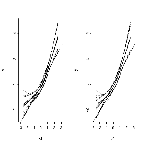
As can be seen, in the left panel, all parameters are shrinked by the same amount a: when df get smaller (i.e. penalty factor gets larger), the regression fit gets flatter and confidence band (dotted curves) become narrower. However, in the right panel, only the cubic spline terms that are nonlinear in X1 are shrinked. Further, as the amount of shrinkage increases (lower df), the fits become more linear and closer to the true regression line (straight dotted line). The stepPlr package provides additional functions for PLME. In particular, the step.plr() function implements L2 penalized logistic regression along with the stepwise variable selection procedure.⁽¹³⁾ Hereafter, I reproduce some of the example code found in the R on-line help.

n <- 100
p <- 10
x <- matrix(rnorm(n*p), nrow=n)
y <- sample(c(0,1), n, replace=TRUE)
fit <- plr(x, y, lambda=1)

First, all predictors appear to be uncorrelated with each other. This was to be expected since the $X_i$ are all random draws from a standard gaussian distribution. The final model is:

$$ \begin{array}{ll} Y & = -0.12434 – 0.22440X_1 + 0.03806X_2 + 0.02807X_3 + 0.10409X_4 \newline &\phantom{{=}} -0.31475X_5 + 0.03531X_6 – 0.05032X_7 + 0.06048X_8 \newline &\phantom{{=}} -0.06450X_9 + 0.04051X_{10} \end{array} $$

Null deviance is estimated to be 137.99 (99 df), while residual deviance is 133.43 (89.9 df). Of course, you will probably obtain different results since it depends on the state of your random generator. If we were to select a more parsimonious variable subset, we might use

step.plr(x,y)

The output indicates that $X_1$, $X_4$ and $X_9\cdot X_1$ have to be included in the final model (Residual deviance now becomes 119.57 on 96 df).

Why stepwise model selection isn’t a good idea?

There are basically three widely used techniques for model selection: forward selection, backward elimination, and stepwise selection. The later can be described in terms of the two other approaches, in particular for the stopping rules:

• Uses both the forward selection and backward elimination criteria.
• Variable selection process terminates when all variables in the model meet the criterion to stay and no variables outside the model meet the criteria to enter.
• Criterion for a variable to enter need not be the same as the criterion for the variable to stay.
• Some advantage in using a more relaxed criterion for entry to force the selection process to consider a larger number of subsets of variables.

Leaps and bounds is another algorithm that was proposed by (9). It allows to find the optimal subset of predictor variables without actually examining all the potential subsets. Its application is limited, however, to subsets of no more than 30 to 50 variables.

So, why not to use stepwise selection? Frank Harrell (Chapter 4, pp. 56-60) provides some clues to the problem of model selection. This “hot topic” is also discussed in several books on regression analysis, including (3) and (4), for example. When using a stepwise procedure for variable selection, one must bear in mind that:

1. It yields R² values that are biased toward higher values.
2. The ordinary F and χ² statistics don’t follow their assumed distribution.
3. Standard errors of regression coefficient estimates are biased low and CI for effects and predicted values are falsely narrow.
4. Regression coefficients are biased toward higher values, calling for shrinkage correction.
5. It yields too liberal P-values due to neglected multiple comparison problems.
6. It does not solve the problem of collinearity (correlation between some of the predictors).

See also these posts compiled by R. Ulrich, and (8). Some authors regard this approach as reveling dredging. In short, stepwise selection, as well as backward and forward procedures, are automated techniques that have to be avoided if one really wants to explore a large set of variables in order to build a confirmatory model. Quoting Harrell (p. 58):

If stepwise selection must be used, a global test of no regression should be made before proceeding, simultaneously testing all candidate predictors and having degrees of freedom equal to the number of candidate variables (plus any nonlinear or interaction terms). If this global test is not significant, selection of individually significant predictors is usually not warranted.

However, when a serious background suggests that some of the variables should be present in the model, stepwise selection could be of interest, though it doesn’t provide a “conservative” way to assess the contribution of a given variable to the model. We are generally looking for a parsimonious model, including primary variables of interest and some other influential factors. In epidemiology, for example, sex, age or tobacco consumption are mandatory variables when modeling some forms of cancer. It would be unbelievable not to include them in a model! With this respect, backward and forward procedures aren’t very recommended when there are plenty of variables since they don’t offer the choice to specify a subset of variables of interest which have to be conserved during the whole selection process.

As proposed by (10), Least Angle Regression⁽¹¹⁾ and the Lasso⁽⁷⁾ techniques offer better alternatives to classical automated selection procedures. Instead of stepwise variable selection algorithm, using methods such as full-model fits or data-reduction ensure a better approach to large-scale model assessment. In particular, the selection of less complex models that are more in agreement with subject matter knowledge should be favored. The Lasso technique is a penalized estimation technique in which the estimated regression coefficients are constrained so that the sum of their scaled absolute values falls below some constant $k$ chosen by cross-validation. Although computationally demanding, this technique offers a way to constrain some regression coefficient to be exactly zero while shrinking the remaining coefficients toward zero. There are several examples of its use in (6), as well as in the R software (see the ElemStatLearn package).

References

1. Ridolfi, A. and Idier, J. (2002). Penalized Maximum Likelihood Estimation for Normal Mixture Distributions. Technical Report IC/2002/85, EPFL.
2. Rousseeuw, P.J. and Yohai, V.J. (1984). Robust regression by means of S-estimators. In J. Franke, W. Härdle, and R.D. Martin (Eds.), Robust and Nonlinear Time Series, Lectures Notes in Statistics, 26 (pp. 256-272). New York: Springer Verlag.
3. Fox, J. (1997). Applied Regression Analysis, Linear Models, and Related Methods.
4. Vittinghoff, E., Glidden, D.V., Shiboski, S.C., and McCulloch, C.E. (2005). Regression Methods in Biostatistics. Springer Verlag. [check my website for additional comments on this book]
5. Alzola, C.F. and Harrell, F.E. (2001). An introduction to S-Plus and the Hmisc and Design Libraries. Electronic book, 299 pages.
6. Hastie, T., Tibshirani, R., and Friedman, J. (2001). The Elements of Statistical Learning. Springer Verlag.
7. Tibshirani, R. (1996). Regression shrinkage and selection via the lasso. Journal of The Royal Statistical Society B, 58(1): 267-288. [check out the dedicated website]
8. Judd, C.M. and McClelland, G.H. (1989). Data Analysis: A Model Comparison Approach. Harcourt Brace Jovanovich.
9. Furnival, G.M. and Wilson, R.W. (1974). Regression by Leaps and Bounds. Technometrics, 16, 499-511.
10. Flom, P.L. and Cassell, D.L. (2007). Stopping Stepwise: Why stepwise and similar selection methods are bad, and what you should use. NESUG 2007 Proceedings.
11. Efron, B., Hastie, T., Johnstone, I., and Tibshirani, R. (2004). Least Angle Regression. The Annals of Statistics, 32(2), 407-499.
12. Shtatland, E.S., Cain, E., and Barton, M.B. (2001). The perils of stepwise logistic regression and how to escape them using information criteria and the Output Delivery System. SUGI 26 Proceedings (pp. 222—226).
13. Park, M.-Y. and Hastie, T. (2006). Penalized Logistic Regression for Detecting Gene Interactions. A modified version of forward-stepwise logistic regression suitable for screening large numbers of gene-gene interactions.