In a previous post, we discussed how influence measures can provide some insights on data quality or model fit. There are various cutoff values that are used to interpret each of these quantities, e.g., $\text{Cook’s d} > 4/(n-k-1)$, $\text{DFFITS} > 2\sqrt{p/n}$, $\text{DFBETAS} > 2/\sqrt{n}$. The latter emphasizes regression coefficients themselves.

Considering a linear predictor $\beta_0 + \sum_{j=1}^k\beta_jx$, the DFBETA value for the $j$th coefficient for the $i$th observation is $\hat\beta_j - \hat\beta_j^{(-i)}$, where $\hat\beta_j^{(-i)}$ is the $j$th coefficient of the regression estimated without the $i$th observation. It’s mostly the jacknife approach to validating a regression model by discarding one observation at a time. From a computational perspective, it is not necessary to compute all $n$ full model since we can rely on linear algebra to relate OLS fit for all $n$ observations to that of any based on $n-1$ observations.¹ Often times, absolute values of DFBETAs are considered instead of signed values, and it is also common to standardize those values since their scale depend on that of the variable of interest. Standardization is done by dividing DFBETAs by the corresponding standard deviation of the $i$th-deleted regression model, and statistical packages often refer to them as DFBETAS instead of DFBETA (note the extra S).

The threshold or reference value, $2/\sqrt{n}$, can be seen as a size-adjusted influence effect accounting for the standard error estimate of the corresponding coefficient. In effect, it amounts to highlight the same theoretical number of influnetial points regardless of sample size, much like when using standardized residuals and referring their distribution to a Student $t$ or $\mathcal{N}$ distribution.

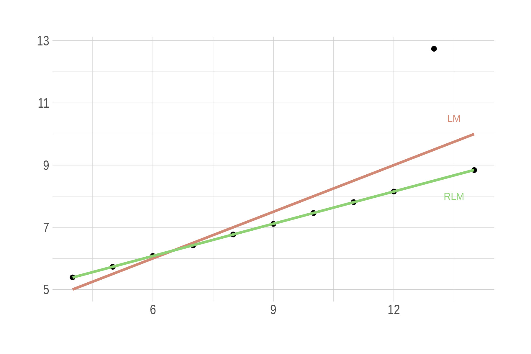
Detecting Influential Points in Regression with DFBETA(S) provides an illustration using simulated datasets of varying size in R. There are some other great articles on the StatLab Archives from the University of Virginia. I am familiar with resistant or robust regression methods (the aforementioned blog post shows how to use DFBETAS to overcome the effect of influential points on a regression line). Here is some old R code illustrating the use of robust regression, as described in Fox & Weisberg on a subset of the Ascombe dataset:

options(hrbrthemes.loadfont=TRUE)
library(MASS)
library(ggplot2)
library(gridExtra)
library(hrbrthemes)
library(directlabels)

set.seed(101)
theme_set(theme_ipsum(base_size = 11))
clr6 = ipsum_pal()(6)

p = ggplot(data = anscombe, aes(x3, y3)) +
  geom_point() +
  geom_smooth(method = "lm", se = FALSE, col = clr6[1]) +
  geom_smooth(method = "rlm", col = clr6[2]) +
  labs(x = NULL, y = NULL) +
  annotate(geom = "text", x = 13.5, y = 10.5, label = "LM", size = 2.8, col = clr6[1]) +
  annotate(geom = "text", x = 13.5, y = 8, label = "RLM", size = 2.8, col = clr6[2])

ggsave("~/fig-lrm-anscombe.png", p3, w = 6, h = 4, dpi = 300)

I just learned about Theil-Sen Regression. Instead of minimizing squared residuals, the slope is calculated by taking the median of the slopes between each pair of points in the data, which basically amounts to compute every possible $(y_j - y_i)/(x_j - x_i)$ if $x_i \neq x_j$.² It follows that the OLS estimate of a simple regression slope can be conceptualized as a weighted average of pairwise slopes, with weights $(x_j - x_i)^2$. Go read the rest of the blog post if you are interested in robust regression.