In one of my answer on Cross Validated I discussed base R solution for diagnosing a regression model. Specifically, I said that “The function influence() (or its wrapper, influence.measures()) returns most of what we need for model diagnostic, including jacknifed statistics. As stated in Chambers and Hastie’s Statistical Models in S (Wadsworth & Brooks, 1992), it can be used in combination to summary.lm(). One of the example provided in the so-called “white book” (pp. 130-131) allows to compute standardized (residuals with equal variance) and studentized (the same with a different estimate for SE) residuals, DFBETAS (change in the coefficients scaled by the SE for the regression coefficients), DFFIT (change in the fitted value when observation is dropped), and DFFITS (the same, with unit variance) measures without much difficulty.”

All of this relies on linear algebra and does not require to perform matrix multiplication or inversions again and again. My impression is that few people really use influence measures (contrary to, say, variance influence factors) even if it may bring some insights into data or model quality. These are simple quantities, though. See one of my old workshop (in French) on statistical modeling (slide #13). For instance, the leverage statistic, or hat value, is defined for observation $i$ as

$$h_i = \frac{1}{n} + \frac{(x_i - \bar x)^2}{\sum_{i=1}^n (x_i - \bar x)^2} = \frac{1}{n} + \frac{(x_i - \bar x)^2}{(n-1)s_x^2}.$$

Note that there is no strict correspondence between outlying and high leverage observations. The mean leverage value is $(k+1)/n$, where $k$ is the number of parameters in the linear model. In the case of simple linear regression, $k=2$. The rule of thumb is that an observation must be carefully checked if $h_i > \frac{2(k+1)}{n}$, which is usually what dedicated statistical packages highlight when asking to print individual diagnostic data.

Fortunately, the Python statsmodels package provides OLSResults.get_influence(), which returns everything we need.

Here is a sample Python script which demonstrates how to compute Cook’s distance¹ from a multiple regression model as illustrated in R’s on-line help for influence.

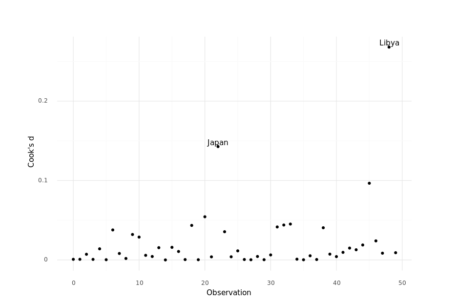
Here are the (filtered) results from R:

        dfb.1_ dfb.pp15 dfb.pp75  dfb.dpi  dfb.ddpi   dffit cov.r   cook.d    hat inf
Japan  0.63987 -0.65614 -0.67390  0.14610  0.388603  0.8597 1.085 1.43e-01 0.2233
Libya  0.55074 -0.48324 -0.37974 -0.01937 -1.024477 -1.1601 2.091 2.68e-01 0.5315   *