In this post I’m going to talk about my adventures with Mathematica as I tackle a small bioinformatics project. The idea is simple: We want to compute the distribution of the distances between SNPs in a VCF file. In fact there are many variant files but once we have a script for one, it can be used for all other files. I think that if you want to master a piece of analysis software, you need to use it as often as possible – and, above all, on real-world projects rather than toy examples, provided it is suited to the task at hand, of course.

The variant file was generated using bcftools as follows:

bcftools query -I ’TYPE="snp""’ -f ‘%CHROM %POS %REF %ALT\n’ strain.allsites.vcf.gz > strain.dist

The strain.allsites.vcf.gz comes from a separate pipeline but suffice it to say that it contains all variants detected for a strain mapped over a reference strain.

Let’s go with the filtered VCF file (strain.dist) which contains only SNPs:

data = Import["strain.dist", "Table"];
sdata = SortBy[data, First];
chrm = SplitBy[sdata, First];

The file is expected to be sorted by contig and by genomic coordinates but it doesn’t cost much to sort things out again before splitting the nested list by contig ID. Indeed, genomic positions are indexed for each contig so the analysis must be carried out for each contig separately. Let’s look a the first contig to see how it goes:

Histogram[Differences[chrm[[1]][[All, 2]]], {50}]

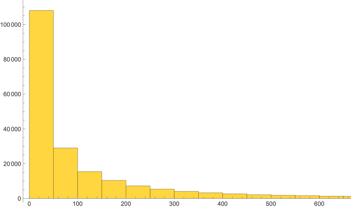
This provides the distribution of succesive differences between each SNP with a bin size of 50 bp. Now, let’s apply this to all contig:

xs = Flatten[Differences[#[[All, 2]]] & /@ chrm];
Histogram[xs, {50}, ImageSize -> Large]

We can do a lot more with empirical distributions in Mathematica. Here for example, we plot the CDF of the empirical distribution (we could also use a SmoothKernelDistribution estimate):

xd = EmpiricalDistribution[xs]
Plot[CDF[xd, x], {x, 0, 1000}, PlotRange -> {All, {0, 1}}]

How does it compare to a Negative Binomial Distribution, with parameters estimated by maximum likelihood from the observed data?

Plot[{CDF[xd, x], 
  CDF[NegativeBinomialDistribution[n, p] /. params, x]}, {x, 0, 500}, 
 Exclusions -> None, PlotStyle -> Thick, PlotRange -> {All, {0, 1}}, 
 PlotLegends -> Placed[{"Empirical", "Model"}, {Right, Bottom}], 
 ImageSize -> Large]

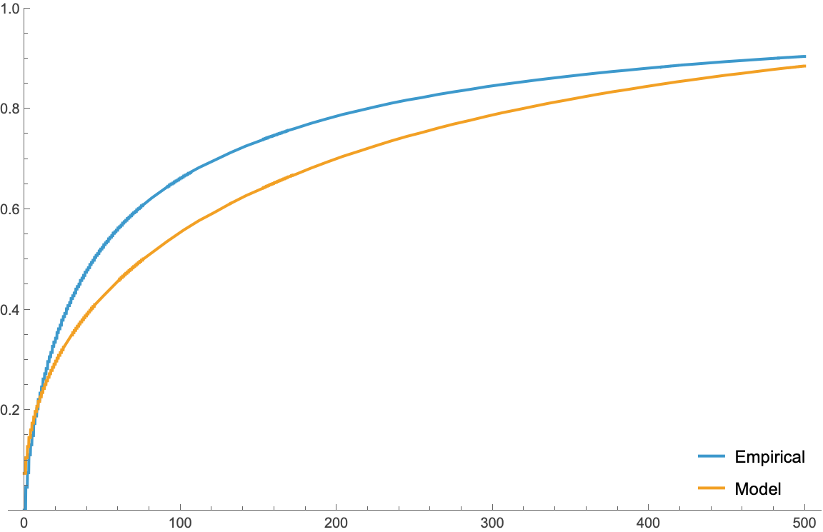
Clearly, there’s a clear departure from the NB distribution in this case, but I hope the above example shows the flexibility of Mathematica when it comes to manipulate empirical and probability distributions. I would have more to say about finding a good-looking PDF for this kind of data, but that should deserve another post.