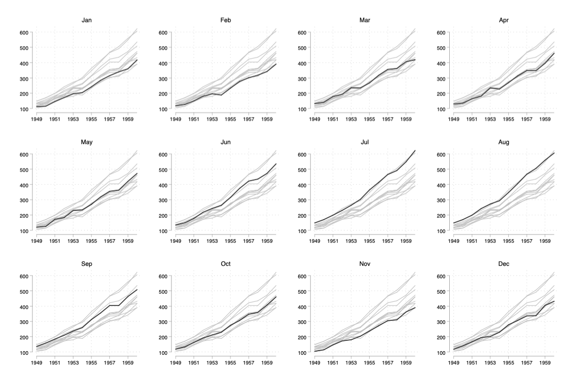
Today, in this new Stata series, we are exploring a variation of small multiples where a separate trend line is highlighted in each subplot while background information is provided in dimmed grey. The final solution makes use of separate, scatter, and graph combine.

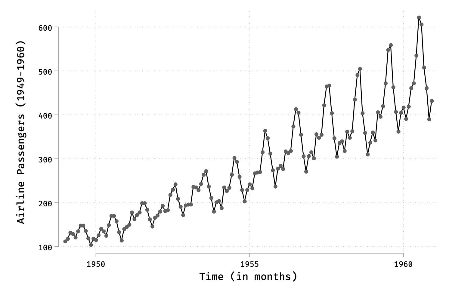
The dataset we will use is composed of 144 observations on the monthly number of international airline passengers (in thousands) between 1949 and 1960. Such time-series dataset would be a perfect fit for a simple line plot, as illustrated below: (Note that I am using the plotplain scheme.)

webuse air2
scatter air time, m(o) c(l)

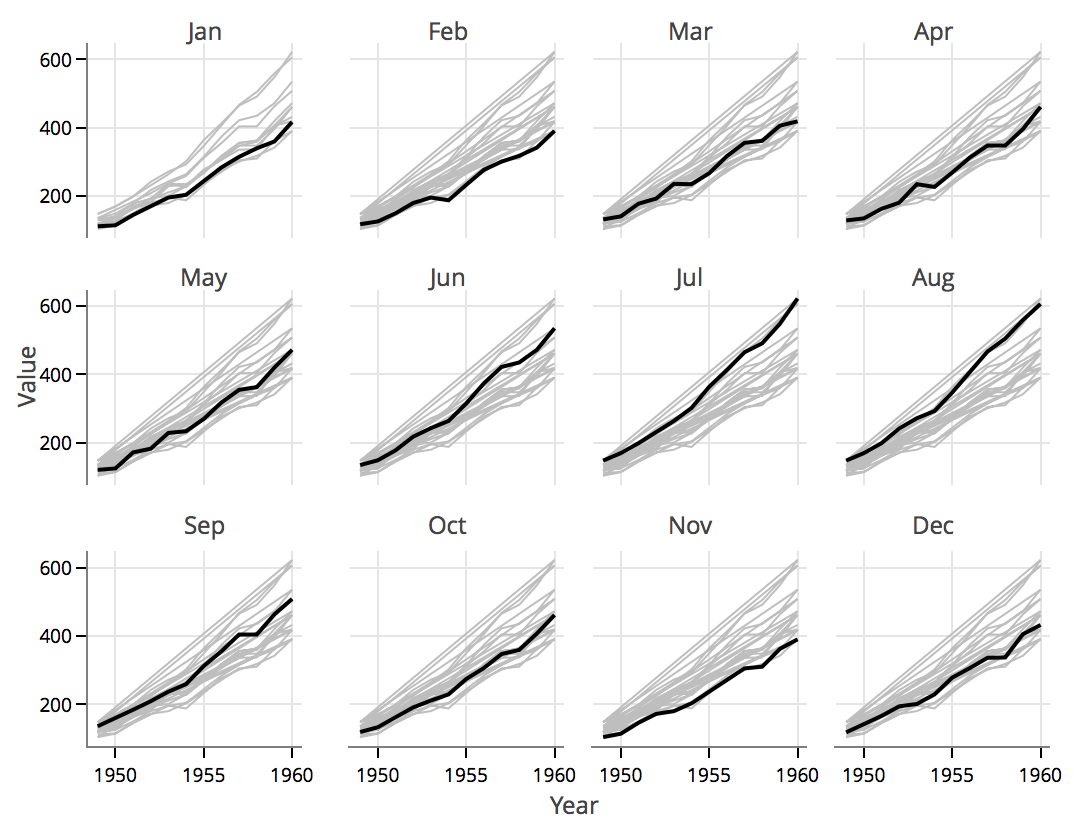
However, what if we want to arrange the data by month but keep a trend line across year? Something like in the following picture, which was made using R:

First, we need to create two new variables that will hold the current month and year, and that will be used for facetting the display:

generate y = floor(time)
generate m = mod(t, 12)
replace m = 12 if m == 0
label define m 1 "Jan" 2 "Feb" 3 "Mar" 4 "Apr" 5 "May" 6 "Jun" 7 "Jul" 8 "Aug" 9 "Sep" 10 "Oct" 11 "Nov" 12 "Dec"
label values m m

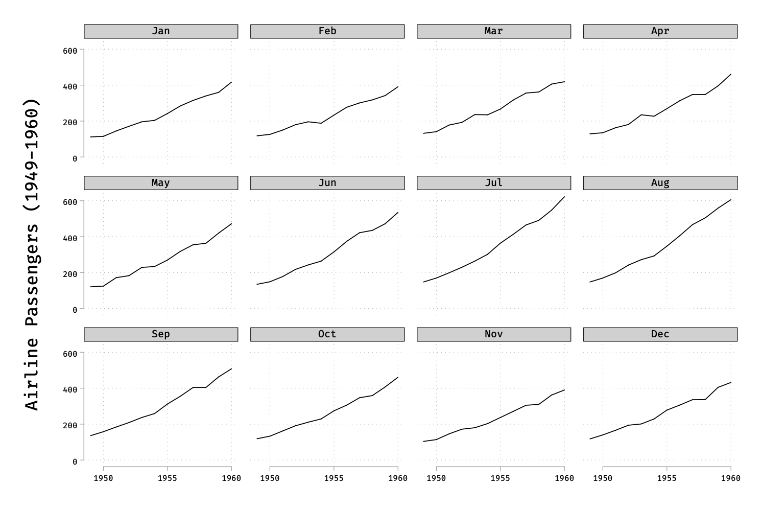
Note that it would be possible to use the creturn value c(Mons) to encode abbreviated month names. This basically allows us to draw yearly data by month as in the following example:

scatter air y, by(m, note("")) c(l) m(none) xtitle("")

The above command could be simplified if we were to rely on time-series (or even panel-related) graphical commands in Stata, e.g.:

tsset m y
tsline air, by(m)

Unfortunately, neither scatter nor tsline offer an over() option, so we must rely on a different approach if we want both an overlay and a facet. There is the sepscatter command, written by Nick Cox, to draw overlaid scatterplots, but it is not a twoway plot type hence it cannot be combined with other twoway commands like scatter. Here is a one-liner command:

sepscatter air y, sep(m) recast(line) lc(gs12 ...) lp(solid ...) legend(off)

It turns out that we can really do the same using a combination of separate and scatter:

separate air, by(m) gen(mm)
scatter mm* y, recast(line) lc(gs12 ...) lp(solid ...) legend(off) || line air y if m == 1, lp(solid) lw(medthick) xtitle("")

Finally, graph combine will allows to combine different graphs into a single file, with the minor caveat that we cannot use regular expression to match graph saved into memory and so we have to list them all (the same problem would happen if we use a saving() option or a graph save command to save graphics on disk). Below is the final command that will be used to generate the final output. Note that we use a for loop to iterate over months for each plot while handling graphic annotation and saving in memory:

forvalues j = 1/12 {
  scatter mm* y, recast(line) lc(gs12 ...) lp(solid ...) xla(1949(2)1960) legend(off) title(mmonth) || line air y if m == `j', lp(solid) lw(medthick) xtitle("") title("`: label m `j''") name(p`j')
}
graph combine p1 p2 p3 p4 p5 p6 p7 p8 p9 p10 p11 p12, rows(3) cols(4)
graph drop _all

The take-away message is that Stata is quite flexible in allowing a by() and an over() option for graphics. When one is not available (e.g., over() in scatter) or cannot be used in combination with other command, one could simply think of an alternate data structure and use graph combine as a replacement of the by() option for facetting.