Stata plot of the week #4

February 10, 2023

This is a continuation of a previous post on building interaction plots in Stata, where I briefly mentioned the margins and marginsplot commands. As I am working on some statistical code as a side project, I need to reproduce a lot of R plots made with ggplot2.

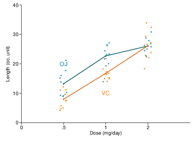
Let’s say we want to reproduce the picture shown at the end of this post. It is a combination of jittered scatterplot with (mean) line plot superimposed. There are surely some Stata packages that are lying around the internet to do this with a magic command, but let’s do this the hard way using built-in commands only. Note that I generally set plotplain as my default color scheme in Stata.¹ So we also need to manage color at some point. But let’s get some data first.

use toothgrowth, clear

summarize

egen dosec = group(dose), label
quietly anova len dosec#supp
quietly margins dosec#supp

At this point, we can use marginsplot directly and start customizing its display options:

marginsplot, noci title("") xtitle(Dose (mg/day)) ytitle(Length (oc. unit)) ///
  addplot(scatter len dosec if supp == 1, ms(oh) jitter(5) ///
  mc(ebblue) text(20 1 "OJ", color(ebblue) size(medlarge)) ///
  xscale(r(0 4)) xlab(0(1)3) || scatter len dosec if supp == 2, ///
  ms(oh) jitter(5) mc(orange) text(10 2 "VC", color(orange) ///
  size(medlarge))) scheme(uncluttered)

In this case, we use the uncluttered color scheme (see also this review of various other schemes on the Stata blog), which gently manages the color for us (although I did not choose the right blue/orange combination in this case).

Here is a similar command built using the menu dialog options for marginsplot, which works with the plotplain scheme:

marginsplot, noci recast(line) ///
  plot1opts(lcolor(ebblue)) plot2opts(lcolor(orange)) ///
  addplot((scatter len dosec if supp == 1, mcolor(ebblue) jitter(5)) ///
  (scatter len dosec if supp == 2, mcolor(orange) jitter(5))) ///
  ytitle(Length (oc. unit)) xtitle(Dose (mg/day)) xscale(range(0.75 3.25)) ///
  title("") legend(off)

I should note taht I was not able to reorder the legend (to suppress the additional keys generated for the scatter added plots) via the menu options. Likewise, I did not bother standardizing the symbol shape as oh. Anyway, this is not hard to fix and both results are shown side by side below:

The anovaplot command works also quite well, actually:

anovaplot dosec supp, scatter(jitter(5))

♪ Rammstein • Amerika

Here is my profile.do configuration by the way:

sysdir set PLUS "~/.local/lib/ado/plus/"
sysdir set PERSONAL "~/.local/lib/ado/personal/"
sysdir set OLDPLACE "~/.local/lib/ado/"

set seed 101
set logtype text
set matastrict on
set maxvar 5000
set scrollbufsize 2000000
set tracedepth 1
// set varabbrev off

set scheme plotplain
graph set eps fontdir ~/.local/share/fonts
graph set window fontface "Roboto Condensed"
if "`c(console)'"!="console" graph set eps preview on
graph set eps logo off
graph set eps fontface "Roboto Condensed"
graph set print logo off
// set autotabgraphs on, perm

set max_memory 8g, permanently

↩︎

aliquote.org

Stata plot of the week #4

See Also