For one of my last lectures I produced the following plot in R:

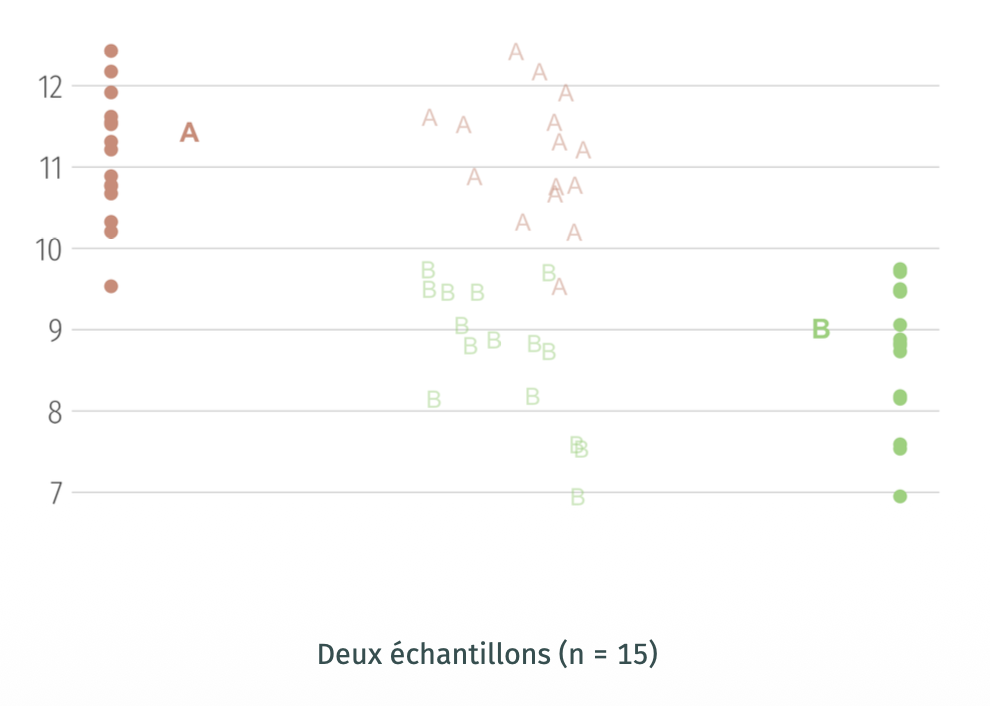
The idea was to illustrate sampling fluctuations and the exchangeability of labels when samples come from the same population, eventually.

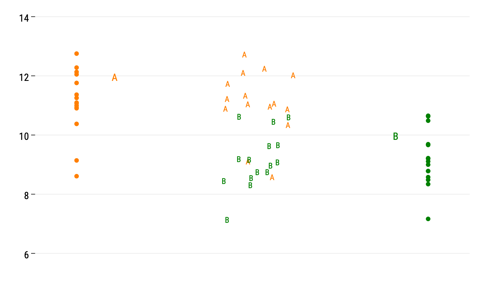
Here’s one way to reproduce this chart using Stata. First, let’s generate two random samples from a Normal distribution with different location parameters:

set seed 101
set obs 15
gen y1 = rnormal(11, 1)
gen y2 = rnormal(9, 1)
gen id = _n
reshape long y, i(id) j(g)
drop id 

Now that we have some data, let’s plot them. Before that, we will need two auxiliary variables:

gen lab = "A"
replace lab = "B" if g == 2
gen mid = 1.5 + runiform(-0.1, 0.1)

The lab will be used for labelling markers while mid will provide jittered position of the x-axis for those markers. We could also use some Stata magic to convert numeric values in g to their corresponding letters, but let’s keep that as simple as possible.

Now for the graphical instructions:

twoway (scatter y g if g == 1, mcolor(orange) text(12 1.1 "A", place(e) color(orange)) ///
  xscale(range(0.9 2.1) noline) yscale(noline) xlabel(, labcolor(bg) tlength(0) nogrid) ///
  ylabel(,grid glp(solid)) xtitle("") ytitle("")) ///
  || (scatter y g if g == 2, mcolor(green) legend(off) text(10 1.9 "B", place(e) color(green))) ///
  || (scatter y mid if g == 1, ms(none) mlabcolor(orange) mlabel(lab)) ///
  || (scatter y mid if g==2, ms(none) mlabcolor(green) mlabel(lab))

Et voilà !