I came across the following puzzle, Expected Tosses for Consecutive Heads: 2 Heads vs 3 Heads Puzzle, this morning:

Let’s say A keep tossing a fair coin, until he get 2 consecutive heads, define X to be the number of tosses for this process; B keep tossing another fair coin, until he get 3 consecutive heads, define Y to be the number of the tosses for this process.

1. Calculate P{X>Y}
2. What’s the expected value of X
3. What’s the expected value of Y

Sure we can enumerate all possible states as the author did. However, we know that $X$ follows a modified Geometrical law: for $k \geq 2$ (we can’t get 2 heads with one trial only) $\Pr(X = k) = \frac{F_{k-1}}{2^k}$, where $F_{k-1}$ is the $k - 1$th term of the Fibonacci series. Assuming a fair coin ($p = 1/2$), the expected number of trials before observing $k = 2$ Heads is given by $2(2^k - 1) = 2^{k+1} - 2$. For $k = 2$ we would need 6 flips.

The transition matrix for the corresponding 3-state Markov chain, where state 0 = 0 consecutive Head, state 1 = 1 consecutive Head, and State 2 = 2 consecutive Heads (absorbing state), is:

$$ \begin{pmatrix} 0.5 & 0.5 & 0 \cr 0.5 & 0 & 0.5 \cr 0 & 0 & 1 \cr \end{pmatrix} $$

Let’s look at the transient states 0 and 1:

$$ Q = \begin{pmatrix} 0.5 & 0.5 \cr 0.5 & 0 \cr \end{pmatrix} $$

The fundamental matrix, $N = (I - Q)^{-1}$, is derived from:

$$ I - Q = \begin{pmatrix} 1 & 0 \cr 0 & 1 \end{pmatrix} - \begin{pmatrix} 0.5 & 0.5 \cr 0.5 & 0 \end{pmatrix} = \begin{pmatrix} 0.5 & -0.5 \cr -0.5 & 1 \end{pmatrix} $$

So that $N = \begin{pmatrix} 4 & 2 \cr 2 & 2 \end{pmatrix}$. The sum of the first row reflects the number of time we will visit state 0 and state 1 before absorption, i.e. 6 flips like we said earlier.

The random variable Y follows a similar law, and the expected number of flips before $k = 3$ Heads therefore is 14.¹

Back to the first question. The probability can be found by summing the joint probabilities: $P(X > Y) = \sum_{y=3}^\infty\sum_{x=y+1}^\infty P(X = x) \cdot P(Y = y)$ (the second lower bound results from the strict inequality constraint, $X > Y$). Or developing the system of equations for all possible joint states like the original author did. Instead of Markov chain analysis, I tried to use the transition matrices and I defined probability distribution in Mathematica as follows:

X = DiscreteMarkovProcess[1, {{1/2, 1/2, 0}, {1/2, 0, 1/2}, {0, 0, 1}}];
Y = DiscreteMarkovProcess[
   1, {{1/2, 1/2, 0, 0}, {1/2, 0, 1/2, 0}, {1/2, 0, 0, 1/2}, {0, 0, 0,
      1}}];
distX = FirstPassageTimeDistribution[X, 3];
distY = FirstPassageTimeDistribution[Y, 4];

The PDFs look okay but Probability[x > y, {x \[Distributed] distX, y \[Distributed] distY}] took way too much time to me. I suspect Mathematica is using symbolic computation under the hood or get lost in an infinite sum. No luck with NProbability either. This is something I have to investigate and I will post an addendum, eventually.

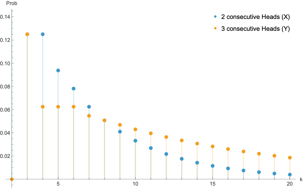
In the meantime, I decided to use a different approach and used Fibonacci and Tribonacci numbers to find the answer quickly, that is by summing the joint probabilities after precomputing sum of the values for X:

trib = RSolveValue[{a[n] == a[n - 1] + a[n - 2] + a[n - 3], a[0] == 0,
     a[1] == 0, a[2] == 1}, a, n];
pdfX[k_] := Fibonacci[k - 1]/2^k;
pdfY[k_] := trib[k - 1]/2^k;
tailX[n_] = 
  FullSimplify[Sum[pdfX[k], {k, n + 1, Infinity}], 
   Assumptions -> n >= 2];
Sum[pdfY[n]*tailX[n], {n, 3, Infinity}] // FullSimplify

We get the expected result, $\frac{361}{1699}$ (0.2125).