Lastly, I came again across a nice poster from Tom Nichols that was presented at the OHBM2010 conference. This was about Finding Distinct Genetic Factors that Influence Cortical Thickness (PDF), and the clustering method that was used is really interesting.

Apart from choosing the right metric, parametric bootstrap was used to assess the stability compactness and separation of clusters as measured with the silhouette width. The need for a validation procedure aims at addressing the following two issues in cluster analysis: (1) bias toward particular cluster properties, and (2) non-significance of results when there’re no true clusters. A more complete review of cluster validation techniques is available in Handl et al. [1].

Basically, the authors established a distinction between three kind of criteria that we want to optimize to get a “good partitioning”: compactness (small within-cluster variation), connectedness (neighbouring data belong to the same cluster), and spatial separation (must be combined with other criteria like compactness or balance of cluster sizes). As part of a large battery of internal measures of cluster validity (i.e., we do not use additional knowledge about the data, like some a priori on class labeling), they can be complemented with so-called combination measures (for example, assessing intra-cluster homogeneity and inter-cluster separation), like Dunn or Davies–Bouldin index, silhouette width, SD-validity index, etc., but also estimates of predictive power (self-consistency and stability of a partitioning), how well distance information are reproduced in the resulting partitions (e.g., cophenetic correlation and Hubert’s Gamma statistic). Ultimately, dedicated measures for correlated data do exist, and this has some obvious applications in genomic studies. Well, there’s much more to read in this paper, especially the benchmark study.

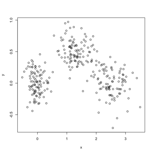
In what follows, I setup a simulation study where I look at the evolution of various validity indices, as well as the cophenetic correlation and average silhouette width following hierarchical clustering. My dataset consists in three well isolated clusters simulated on a 2D plane, as follows:

sim.xy <- function(n, mean, sd) cbind(rnorm(n, mean[1], sd[1]),
rnorm(n, mean[2],sd[2]))
xy <- rbind(sim.xy(100, c(0,0), c(.2,.2)),
            sim.xy(100, c(2.5,0), c(.4,.2)),
            sim.xy(100, c(1.25,.5), c(.3,.2)))

Here is how it looks:

(I generally fix my seed at a value of 101 if one is interested in reproducing the results.)

Then, the main loop just capture the relevant output from cluster.stats in the fpc package. Silhouette widths are computed from the cluster package:

dat <- xy
n <- nrow(dat)
B <- 20
k <- seq(2,20)
stat <- c("avg.silwidth", "g2", "g3", "pearsongamma", "dunn", "ch",
          "within.cluster.ss", "wb.ratio")
res.hc2 <- array(dim=c(B, length(k), length(stat)),
                 dimnames=list(1:B, k, stat))
for (b in 1:B) {
  cat("Iteration ", b, "\n")
  tmp <- dat[sample(1:n, n, replace=TRUE), ]
  dd <- dist(tmp)
  hc <- hclust(dd, method="ward")
  for (i in k)
    res.hc2[b,i-1,] <- as.numeric(unlist(cluster.stats(dd, 
    cutree(hc, i), G2=TRUE, G3=TRUE)[stat]))
}

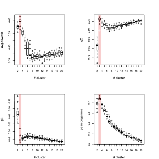
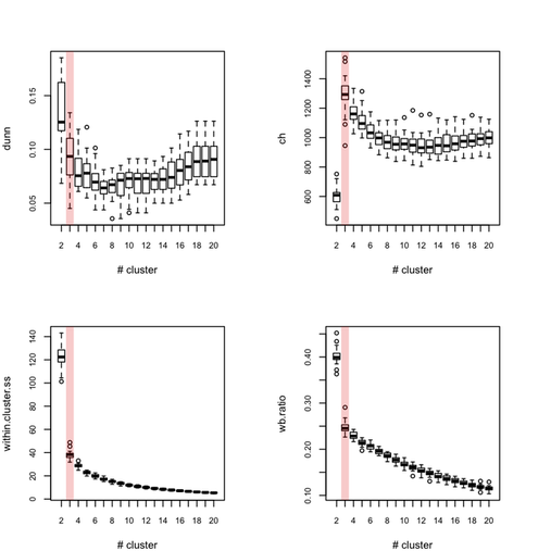
Each outer loop tooks about 2'30 to complete so this is rather long, but I haven’t much time to invest in optimizing or distributing the code. Obviously, this would be better to use, say 100 or 500 boostrap samples. Anyway, here are the results for all eight indices, where the “true” number of clusters is highlighted in red.

Below (left) I show a complete experiment on 500 bootstrap samples, when just estimating average silhouette width for a varying number of clusters:

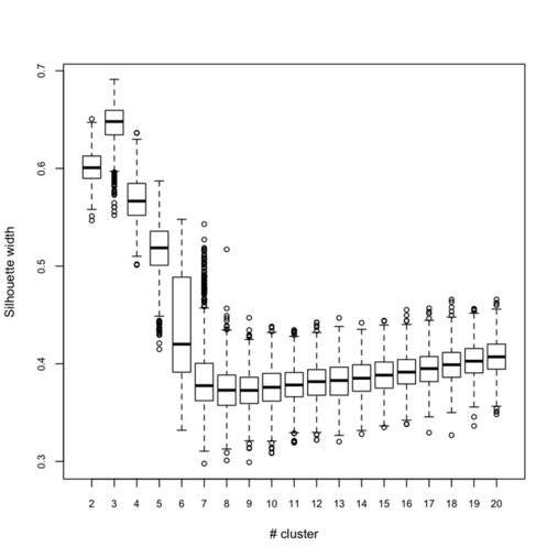
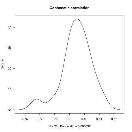
Clearly, the maximal value is reached for $k = 3$, and we can observe that when $k = 6$ there’s a large variability in silhouette widths, whereas for k > 7 the results are monotonically increasing with few within-essay variability. For the same experiment, the cophenetic correlation exhibits the following variations:

  Min. 1st Qu.  Median    Mean 3rd Qu.    Max. 
0.7678  0.7900  0.7951  0.7947  0.8006  0.8123 

Its distribution is displayed in the preceding figure on the right.

So, what can we conclude from this? Overall, the silhouette criteria, as well as G2 and G3 indices work well, although in the latter case it is difficult to tell whether its extremal value really distinguishes from simple noise (we would need more bootstrap samples, probably). The Dunn index is not that reliable as it highlights a very large variance at the optimal solution. The within-cluster SS, and consequently the within- and between-SS ratio show a clear pattern (exponential decrease when increasing the number of clusters), although in this particular case it might well be explained by the characteristic distributions chosen for our 2D clouds of points. Finally, the Calinksy criteria seems to work too, although with high variance. But I have had varying experience with its use a quality of clustering measure because it largely depends on the balance in cluster size.

I replicate cluster analysis using the k-means algorithm and the Gap statistic for selecting the number of clusters. There was a package, SLmisc, that handled all that but it not on CRAN anymore. It needs to be installed by hand. So basically, I choose 10 random starting configuration and let the algorithm stop when $\text{Gap}(k) - \text{Gap}(k+1) + s(k+1) \ge 0$ (where $s(k+1)$ is the standard error of the simulated results) or k.max=10 is reached, which never happened. The results are shown in the next figure, on the left:

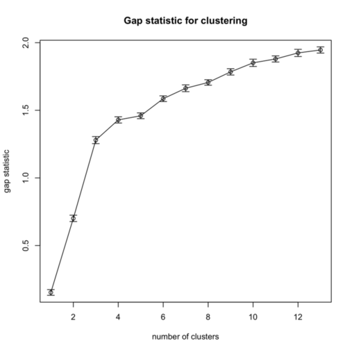
As can be seen, using the “elbow criteria” would lead to retain a three-cluster solution.

Finally, turning back to hierarchical clustering, I also tried the clusterboot() function from the fpc package. As described in Hennig [3] and the on-line help:

Assessment of the clusterwise stability of a clustering of data, which can be cases*variables or dissimilarity data. The data is resampled using several schemes (bootstrap, subsetting, jittering, replacement of points by noise) and the Jaccard similarities of the original clusters to the most similar clusters in the resampled data are computed. The mean over these similarities is used as an index of the stability of a cluster (other statistics can be computed as well).

The syntax I used was:

hc.boot <- clusterboot(dist(xy), B=20, bootmethod="boot",
                       clustermethod=disthclustCBI, method="ward", 
           cut="number", k=3, showplots=TRUE)

All images were saved as separate PNGs, and then converted to an animated GIF with ImageMagick. It would have been better to set fixed values for the x- and y-axis ticks, though. The result is displayed above (right panel).

Number of clusters found in data:  3 

 Clusterwise Jaccard bootstrap mean:
[1] 1.0000000 0.9192952 0.9193784
dissolved:
[1] 0 0 0
recovered:
[1] 20 20 20

As can be seen, the Jaccard similarity value is largely above 0.90, which means that resampled units are generally found to belong to the same cluster.

There are many other settings that might be explored; I can think of: varying the sample size, varying the shape of the variance-covariance matrices, using a larger number of variables and pre-process them with some kind of feature selection algorithm, etc.

References

1. Handl, J., Knowles, J., and Kell, D.B. (2005). Computational cluster validation in post-genomic data analysis. Bioinformatics, 21(15): 3201-3212.
2. Giancarlo, R., Scaturro, D., and Utro, F. (2008). Computational cluster validation for microarray data analysis: experimental assessment of Clest, Consensus Clustering, Figure of Merit, Gap Statistics and Model Explorer. BMC Bioinformatics, 9: 462.