Just a quick note for myself, since I don’t use that often but I may forget it once again (like I did before). The R connector, RLink, was introduced in Mathematica v9, if I remember correctly, it was sometimes a pain in the ass to use it properly, but now things seem to go smoothly once you get the right setup, although you may get some occasional crashed which require that you perform the install step again (this is just the first instruction below).

Working environment: Ubuntu 22.04 LTS, R 4.3.2, Mathematica 13.3.

First, we need to ensure that RLink is actually working (you’ll likely need to install rJava from R, which is a required step to get a working Java link):¹

In[59]:= InstallR["RHomeLocation" -> "/usr/lib/R"]

If everything went fine, you can check which version of R was linked to the active session:

In[60]:= REvaluate["R.version.string"]
Out[60]= {"R version 4.3.2 (2023-10-31)"}

Then, in order to pass data structure from Mathematica to R, we need to use RSet and pass both the Mathematica object and an internal name that will be recognized when subsequently evaluating R code.² We can then use REvaluate or type > at the prompt to get an evaluation cell targeting Julia, Python, Octave, R, and many other DSLs.

Here is a working example where we use bootstrap resampling and distribution fitting using Mathematica builtins and R’s venerable fitdistr from the MASS package.

In[53]:= data={7.05,2.49,16.09,21.3,19.21,14.88,16.41,0.19,9.71,10.18,8.81,
            2.93,18.11,22.2,9.79,14.74,4.54,16.76,8.46,24.9};
         Skewness[data]
Out[54]= -0.0333154
In[42]:= skews=Table[Skewness[RandomChoice[data,Length[data]]],{1000}];
In[44]:= StandardDeviation[skews]
Out[44]= 0.333235

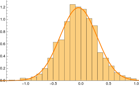
The histogram for the sampling distribution of the skewness (1000 bootstrap samples) is shown on the left, together with the best fitting gaussian PDF:

The density estimator was obtained as follows:

dist=EstimatedDistribution[skews, NormalDistribution[mu,sigma]];
Show[Histogram[skews, Automatic, "PDF"], Plot[PDF[dist, x], {x, -2, 2}, PlotStyle->Orange]]

We can also use FindDistributionParameters to find the MLE assuming a gaussian distribution; moreover, we could rely on bootstrap to perform the same estimation.

In[67]:= FindDistributionParameters[skews,NormalDistribution[\[Alpha],\[Beta]]]
Out[67]= {\[Alpha]->-0.0460534,\[Beta]->0.333068}

Now let’s estimate the parameters of the normal distribution from the data using R:

In[73]:= RSet["skews", skews];
In[74]:= fit = MASS::fitdistr(skews, "normal")
Out[74]= RObject[{RObject[{-0.0460534,0.333068},RAttributes[names:>{mean,sd}]],RObject[{0.0105325,0.00744763},RAttributes[names:>{mean,sd}]],RObject[{{0.000110934,0.},{0.,0.0000554671}},RAttributes[dimnames:>{{mean,sd},{mean,sd}}]],{1000},{-319.53}},RAttributes[names:>{estimate,sd,vcov,n,loglik},class:>{fitdistr}]]
In[78]:= sd(skews)
Out[78]= {0.333235}

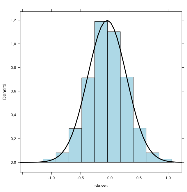
There are some convenient functions to get a prettier display of the results, but let’s note that with R the mean and standard deviation are estimated as -0.0460534 and 0.333068, which comparable to the values estimated by Mathematica. Since Rlink is systematically crashing with ggplot2, I will resort on lattice to display an histogram of the data together with a density plot.

In[110]:= REvaluate["library(lattice)"]
Out[110]= {lattice,stats,graphics,grDevices,utils,datasets,methods,base}
In[112]:= print(histogram(~ skews, data = data.frame(skews),
                   type = "density",
                   panel=function(x, ...) {
                      panel.histogram(x, col = "lightblue", ...)
                      panel.mathdensity(dmath=dnorm, args=list(mean=-0.0460534, sd=0.333068),
                                        col = "black", lwd = 3, ...)
               }))

The result is shown in the right panel of the above figure.