Apart from summarizing some notes I took when reading articles and book chapters about Random Forests (RF), I would like to show some simple way to graphically summarize how RFs work and what results they give.

Some time ago, there was a question on stats.stackexchange.com about visualizing RFs output. Well, in essence the responses were that it is not very useful as a single unpruned tree is not informative about the overall results or classification performance. Yet, there may be some cases where showing how trees are built and how similar they are might be of interest, especially for the researcher or physician who isn’t that used to ML techniques. Although I will not provide a working illustration to this specific question, we can still play with simple decision trees and shuffle the dataset onto which they are evaluated. In short, we can apply some sort of bagging.

Some properties of RF

Why are RFs so attractive now? Basically, RFs retain many benefits of decisions trees while achieving better results and competing with SVM or Neural Networks. In short, RFs handles missing values and mixed type of predictors (continuous, binary, categorical); it is also well suited to high-dimensional data set, or the $n \ll p$ case. Contrary to classical decision tree, there is no need to prune the trees (to overcome overfitting issues) because the RF algorithm takes care of providing bias-free estimate of test error rate.

There are indeed two levels of randomization: first, we select a random subset of the available individuals, then we select a random subset of the predictors (typically, $\sqrt{k}$ or $k/3$, for classification and regression, respectively). It is also worth noting that RFs can be used in unsupervised as well as supervised mode.

In contrast, pruning must be used with decision trees to avoid overfitting: this is done by achieving a trade-off between complexity (i.e., tree size) and goodness of fit (i.e., node impurity). Decision trees are only applicable within a supervised context.

In addition to the dedicated website, here are important publications by Leo Breiman and coll.:

• Breiman, L, Friedman, J, Olshen, R, and Stone, C. (1984). Classification and Regression Trees. Chapman & Hall.
• Breiman, L. (1996). Bagging predictors. Machine Learning, 26, 123-140.
• Breiman, L. (2001). Random Forests. Machine Learning, 45(1), 5-32.
• Breiman, L. (2001). Statistical modeling: The two cultures. Statistical Science, 16(3), 199-231.

Some recent articles or chapter books are also given in the references section.

The main features of RFs are that we end up with estimates for

1. the test error, through the use of out-of-bag samples (this is basically how bagging works: just select with replacement a subset of all individuals) and a majority vote (classification) or average (regression) scheme;
2. the importance of each predictor, by randomly permuting the predictors and computing the increase in OOB estimate of the loss function;
3. the measure of individuals proximity, by keeping track of the number of times any two samples $x_i$ and $x_j$ end up in the same terminal node.

We said that RFs share some resemblance with bagging, but this is not the case of boosting. With boosting, we would consider all features at the same time (and not a subset thereof), and tree building would be chained, whereas in RF each tree are built independently one to the other. This is particularly interesting because it means that the RF algorithm can benefit from parallelization. Moreover, with high-dimensional data set where the number of predictors is largely over the number of samples, boosting will be slower compared to RF. A well-known example of boosting is Gradient Boosting Machine. For further discussion, please refer to Chapter 10 of The Elements of Statistical Learning that should makes it clear that Boosting has few to do with bagging. It is also worth noting that some authors argued that RFs actually perform as well as penalized SVM or GBM.⁽¹⁾

An illustration of bagging with classification trees

We will use the randomForest R package, which conforms to the original algorithm proposed by Breiman.

Here is how we fit an RF model to the well-known iris dataset:

data(iris)
library(randomForest)
set.seed(71)
iris.rf <- randomForest(Species ~ ., data=iris, importance=TRUE)
print(iris.rf)

And here are the results:

               Type of random forest: classification
                     Number of trees: 500
No. of variables tried at each split: 2

        OOB estimate of  error rate: 4.67%
Confusion matrix:
           setosa versicolor virginica class.error
setosa         50          0         0        0.00
versicolor      0         47         3        0.06
virginica       0          4        46        0.08

Now, let’s look at the following code. First, we select a random sample of units, of the same size as the original dataset, but with replacement, so that approximately 1/3 of the samples will not be present (they serve as out-of-bag individuals):

n <- nrow(iris)
selidx <- sample(1:n, n, replace=TRUE)

In my case, length(unique(selidx)) returns 93 which means that 62% of the statistical units are present in this sample:

require(tree)
t1 <- tree(Species ~ ., data = iris[selidx,])
summary(t1)

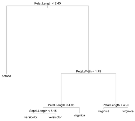
Here are the results for this tree:

Classification tree:
tree(formula = Species ~ ., data = iris[selidx, ])
Variables actually used in tree construction:
[1] "Petal.Length" "Petal.Width" 
Number of terminal nodes:  4 
Residual mean deviance:  0.06548 = 9.561 / 146 
Misclassification error rate: 0.02 = 3 / 150 

Note that instead of tree(), we could have used the rpart package. The resulting tree looks like the one shown below:

Well, what about doing this 50 times, each time with a different base sample?

k <- 10
WD <- "~/tmp/"
fps <- 25
for (i in 1:k) {
  t <- tree(Species ~ ., 
            data = iris[sample(1:n, n, replace=TRUE),])
  png(paste(WD, formatC(i, digits=3, flag="0"), ".jpg", sep=""))
  plot(t, col="gray"); text(t, cex=.8)
  dev.off()
}

We can then assemble all jpg into a movie like this (with ImageMagick):

$ convert -delay 10 *.jpg bagging.mpg
$ ffmpeg bagging.mpg bagging.mov

Here is the result:

As can be seen, the cutoff considered for splitting each node varies from one trial to the other, but overall the tree structure appears to be relatively stable (well, this is also a school case). It should be noted that we didn’t consider a random subset of the variables of interest when growing a tree, and that we don’t collect class membership predicted on OOB data. Finally, we don’t apply the permutation scheme used in RF to assess variable importance, so this really is a toy example, but it can be extended without any difficulties. In particular, there is a tree extractor in the randomForest package, see help(getTree). Note that it is a raw data frame, so we still need to build a wrapper function around that information to produce an object of class tree.

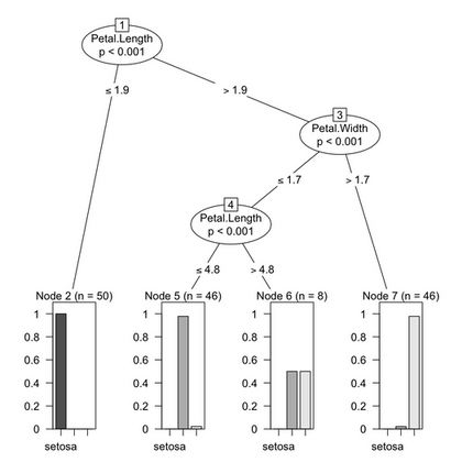
There are a lot of other packages to explore, including: party, maptree, marginTree, psychotree, boruta, caret, longRPart, ipred. The above results might be contrasted with, for instance, those obtained from the ctree() from the party package. Quoting the vignette, “The conditional distribution of statistics measuring the association between responses and covariates is the basis for an unbiased selection among covariates measured at different scales. Moreover, multiple test procedures are applied to determine whether no significant association between any of the covariates and the response can be stated and the recursion needs to stop.”

Although we didn’t prune our trees in the preceding example, using ctree() alleviates the need of bothering with that. In effect, tree growth is governed by statistical stopping rules (see section 3 of the vignette, party: A Laboratory for Recursive Partytioning).

Carolin Strobl gave a nice talk during the UseR! 2008 conference on variable importance: Why and how to use random forest variable importance measures (and how you shouldn’t). I seem to remember that she also presented the cparty package at the IMPS 2009 conference.

Further Notes

The KLIMT software may also be used to visualize trees. We could try to reproduce the above example with the iris data (see iris.full, 11 Kb).

I came across another implementation of RF last year. This is called Random Jungle, and it seems to be dedicated to high-dimensional data. I didn’t try it yet. A priori, there’s no binary for OS X, and it relies on the Boost and GSL libraries; provided you have both installed on your system, you could run

./configure --with-boost=/usr/local/share/boost
make

I had a problem with default build rules that target both i386 and x86_64 arhitectures. I used only one and add the -m64 switch to gcc, g++ and gfortran. Be aware that it should match your GSL installation, but you can still disable GSL support during configure.

For further information, please refer to the documentation, and have a look at the original article: Schwarz, D.F., König, I.R., and Ziegler, A. (2010). On safari to Random Jungle: a fast implementation of Random Forests for high-dimensional data. Bioinformatics, 26(14), 1752-1758.

The documentation has some illustrations of use with R and plink.

Here are the results I got when applying this algorithm on the “iris” data. Data were exported into a flat file as suggested in the documentation:

data(iris)
mydata <- iris
mydata$Species <- as.integer(mydata$Species) # convert factor to integer
write.table(mydata, file="data_from_r.dat", row.names=FALSE, quote=FALSE)

Then, I launched the program as follows:

$ rjungle  -f data_from_r.dat -U1 -z1 -t500 -v -D Species -o example4
         Start: Fri Feb 25 21:10:00 2011
+---------------------|-----------------|-------------------+
|    RandomJungle     |      1.2.363    |        2011       |
+---------------------|-----------------|-------------------+
|    (C) 2008-2011 Daniel F Schwarz et al., GNU GPL, v2     |
|           daniel@randomjungle.com                         |
+-----------------------------------------------------------+

Output to: example4.*
Loading data... 
Read 150 row(s) and 5 column(s).
Use 150 row(s) and 5 column(s).
Dependent variable name: Species
Growing jungle...
Number of variables: 5 (mtry = 2)
1 thread(s) growing 500 tree(s)
Growing time estimate: ~0 sec.
progress: 10%
progress: 20%
progress: 30%
progress: 40%
progress: 50%
progress: 60%
progress: 70%
progress: 80%
progress: 90%
Generating and collecting output data...
Writing accuracy information...
Calculating confusion matrix...

Growing time: 0.184852 sec
Elapsed time: 0 sec
Finished: Fri Feb 25 21:10:00 2011

The confusion matrix is shown below:

$ cat example4.confusion
Iteration: 0
Number of variables: 5
Test/OOB set: 
(real outcome == rows / predicted outcome == columns )	
    1	2	3	error
1	50	0	0	0
2	0	47	3	0.06
3	0	4	46	0.08
                0.0466667

How nice, isn’t it?

References

1. Cutler, A., Cutler, D.R., and Stevens, J.R. (2009). Tree-Based Methods, in High-Dimensional Data Analysis in Cancer Research, Li, X. and Xu, R. (eds.), pp. 83-101, Springer.
2. Saeys, Y., Inza, I., and Larrañaga, P. (2007). A review of feature selection techniques in bioinformatics. Bioinformatics, 23(19):2507.
3. Díaz-Uriarte, R., Alvarez de Andrés, S. (2006). Gene selection and classification of microarray data using Random Forest. BMC Bioinformatics, 7:3.
4. Díaz-Uriarte, R. (2007). GeneSrF and varSelRF: a web-based tool and R package for gene selection and classification using Random Forest. BMC Bioinformatics, 8:328.
5. Sutton, C.D. (2005). Classification and Regression Trees, Bagging, and Boosting, in Handbook of Statistics, Vol. 24, pp. 303-329, Elsevier.
6. Moissen, G.G. (2008). Classification and Regression Trees. Ecological Informatics, pp. 582-588.
7. Geurts, P., Ernst, D., and Wehenkel, L. (2006). Extremely randomized trees. Machine Learning, 63(1), 3-42.

(I should have something like 50+ papers on the use of RFs in various settings; I will put a BibTeX file somewhere when I had time.)