The data have to be loaded in the workspace first. This can be done as
follows:
> WCGS <- read.table("wcgs.txt",header=TRUE,sep="\t")
> WCGS\$arcus_f <- as.factor(WCGS\$arcus)
> WCGS.lm1 <- lm(chol~arcus_f,data=WCGS)
> summary(WCGS.lm1)
Call:
lm(formula = chol ~ arcus_f, data = WCGS)

Residuals:
     Min       1Q   Median       3Q      Max
-119.906  -28.906   -2.906   27.094  422.094

Coefficients:
            Estimate Std. Error t value Pr(>|t|)
(Intercept) 222.9060     0.9186 242.652  < 2e-16 ***
arcus_f1     11.5140     1.6807   6.851 8.82e-12 ***
---
Signif. codes:  0 '***' 0.001 '**' 0.01 '*' 0.05 '.' 0.1 ' ' 1

Residual standard error: 43.11 on 3138 degrees of freedom
  (14 observations deleted due to missingness)
Multiple R-Squared: 0.01474,    Adjusted R-squared: 0.01442
F-statistic: 46.93 on 1 and 3138 DF,  p-value: 8.816e-12
So, we can see that mean effect is estimated to be 11.5: This is the
difference between response measured for level 1 and level 0 of the arcus
factor. In this case, the intercept is simply the baseline value, that is the
mean response for level 0.
Now, if we relevel the factor such that reference level becomes level 1, we
will see a different pattern of results:
> levels(WCGS\$arcus_f)
[1] "0" "1"
> WCGS\$arcus_f2 <- relevel(WCGS\$arcus_f,"1")
> levels(WCGS\$arcus_f2)
[1] "1" "0"
> WCGS.lm2 <- lm(chol~arcus_f2,data=WCGS)
> summary(WCGS.lm2)
Call:
lm(formula = chol ~ arcus_f2, data = WCGS)

Residuals:
     Min       1Q   Median       3Q      Max
-119.906  -28.906   -2.906   27.094  422.094

Coefficients:
            Estimate Std. Error t value Pr(>|t|)
(Intercept)  234.420      1.407 166.552  < 2e-16 ***
arcus_f20    -11.514      1.681  -6.851 8.82e-12 ***
---
Signif. codes:  0 '***' 0.001 '**' 0.01 '*' 0.05 '.' 0.1 ' ' 1

Residual standard error: 43.11 on 3138 degrees of freedom
  (14 observations deleted due to missingness)
Multiple R-squared: 0.01474,    Adjusted R-squared: 0.01442
F-statistic: 46.93 on 1 and 3138 DF,  p-value: 8.816e-12
> with(WCGS, tapply(chol,arcus_f,mean,na.rm=T))
       0        1
222.9060 234.4200
> with(WCGS, tapply(chol,arcus_f2,mean,na.rm=T))
       1        0
234.4200 222.9060
> table(WCGS\$arcus_f2)

   1    0
 941 2211
At present, Intercept takes the mean response for the reference value (234.4)
while the (negative) slope represents the mean difference between the two
conditions.
Obviously, regarding the slope paramater, this recoding doesn't affect other
aspect of estimation procedure, such as standard error (indeed, they are the
same in the two models), confidence interval, or associated p-value. However,
we will notice some difference for the intercept, since `beta`0 takes a
different value and is estimated on a different sample size (941 instead of
2211): As a consequence of reduced n, SE will be increased, and t-value will
be decreased.
Finally, note that we will get strictly the same results when treating arcus
as a quantitative variable (results not shown), when using 0/1
coding. However, this will not hold if we recode the 0/1 value as 1/2. Indeed,
if our variable now takes only two integer values, ranging form 1 to 2, both
the intercept and slope parameters will differ from what was observed in the
preceding. It results from simple geometrical consideration about the
estimation of slope and intercept in linear regression with continuous outcome
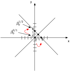
and predictor [Fig. 1].
> WCGS\$arcus2 <- WCGS\$arcus
> WCGS\$arcus2[WCGS\$arcus2==0] <- 2
> WCGS.lm3 <- lm(chol~arcus2,data=WCGS)
> summary(WCGS.lm3)
Call:
lm(formula = chol ~ arcus2, data = WCGS)

Residuals:
     Min       1Q   Median       3Q      Max
-119.906  -28.906   -2.906   27.094  422.094

Coefficients:
            Estimate Std. Error t value Pr(>|t|)
(Intercept)  245.934      2.961  83.056  < 2e-16 ***
arcus2       -11.514      1.681  -6.851 8.82e-12 ***
---
Signif. codes:  0 '***' 0.001 '**' 0.01 '*' 0.05 '.' 0.1 ' ' 1

Residual standard error: 43.11 on 3138 degrees of freedom
  (14 observations deleted due to missingness)
Multiple R-Squared: 0.01474,    Adjusted R-squared: 0.01442
F-statistic: 46.93 on 1 and 3138 DF,  p-value: 8.816e-12
First, we notice that the sign of the slope coefficient has been reversed, as
before (releveling the categorical variable). Meanwhile, the value for
intercept is now 245.9 (vs. 222.9 for the 0/1 coding) and its standard error
is three times that obtained using 0/1 coding (result not shown). Wherefore
such a difference? As can be seen from the following figure, in the case of a
linear regression where slope is estimated to be unity (and we are considering
centered variable for the purpose of the illustration), reversing the values
taken by X “move” the relation in the opposite direction: Slope become -1
while intercept is twice the preceding (precisely, `beta`0 times
(x2-x1)).
Figure 1: A simple illustration of regression slope estimation in the continuous case.
Other coding scheme could be considered, for example (-1,+1) for the two
level. In this case, the difference between the two level would be largely
decreased, as can be seen in the following:
> WCGS\$arcus3 <- WCGS\$arcus
> WCGS\$arcus3[WCGS\$arcus==0] <- -1
> WCGS.lm5 <- lm(chol~arcus3,data=WCGS)
> summary(WCGS.lm5)
Call:
lm(formula = chol ~ arcus3, data = WCGS)

Residuals:
     Min       1Q   Median       3Q      Max
-119.906  -28.906   -2.906   27.094  422.094

Coefficients:
            Estimate Std. Error t value Pr(>|t|)
(Intercept) 228.6630     0.8404 272.098  < 2e-16 ***
arcus3        5.7570     0.8404   6.851 8.82e-12 ***
---
Signif. codes:  0 '***' 0.001 '**' 0.01 '*' 0.05 '.' 0.1 ' ' 1

Residual standard error: 43.11 on 3138 degrees of freedom
  (14 observations deleted due to missingness)
Multiple R-Squared: 0.01474,    Adjusted R-squared: 0.01442
F-statistic: 46.93 on 1 and 3138 DF,  p-value: 8.816e-12
If we consider again the output of lm(chol~arcus,data=WCGS), we can get the
fitted value with the predict or fitted functions.
> yhat <- fitted(WCGS.lm3)
> length(yhat)
[1] 3140
> length(WCGS\$chol[!is.na(WCGS\$arcus)])
[1] 3152
Note, however, that the length of vector of fitted values differ from what is
expected. This comes from the fact that some observations were removed before
fitting the model.
> print(idx <- attr(WCGS.lm3\$model,"na.action"))
  97  494  619  746  910 1273 1661 1847 2113 2222 2358 2605 2613 3047
  97  494  619  746  910 1273 1661 1847 2113 2222 2358 2605 2613 3047
attr(,"class")
[1] "omit"
We can now estimate the squared correlation between the two vectors and
compare it to R2.
> cor(yhat,WCGS\$chol[-as.numeric(idx)])^2
[1] 0.01473513
> summary(WCGS.lm3)\$r.squared
[1] 0.01473513
Recall from
Chapter 4
that the effect of physical activity on glucose level has been considered as
significant based on overall model fit and individual comparison (linear
contrasts `beta`0 `+` `beta`2 = 0 and -`beta`3 + `beta`5 = 0).
> HERS <- read.table("hersdata.txt",header=TRUE,na.strings=".")
> HERS$physactf <- as.factor(HERS$physact)
> physact.desc <- c("1=Much less active","2=Somewhat less active",
+ "3=About as active","4=Somewhat more active","5=Much more active")
> HERS.lm <- lm(glucose~physactf,data=HERS,subset=diabetes==0)
> summary(HERS.lm)
Call:
lm(formula = glucose ~ physactf, data = HERS, subset = diabetes ==
    0)

Residuals:
     Min       1Q   Median       3Q      Max
-48.9867  -6.9867  -0.9867   5.8056  29.8571

Coefficients:
            Estimate Std. Error t value Pr(>|t|)
(Intercept)  98.4206     0.9393 104.784   <2e-16 ***
physactf2    -0.8584     1.0842  -0.792   0.4286
physactf3    -1.2262     1.0111  -1.213   0.2254
physactf4    -2.4339     1.0108  -2.408   0.0161 *
physactf5    -3.2777     1.1211  -2.924   0.0035 **
---
Signif. codes:  0 *** 0.001 ** 0.01 * 0.05 . 0.1   1

Residual standard error: 9.716 on 2027 degrees of freedom
Multiple R-squared: 0.008668,  Adjusted R-squared: 0.006712
F-statistic: 4.431 on 4 and 2027 DF,  p-value: 0.001441
> confint(HERS.lm)
                2.5 %      97.5 %
(Intercept) 96.578530 100.2625914
physactf2   -2.984617   1.2677189
physactf3   -3.209060   0.7566629
physactf4   -4.416114  -0.4515950
physactf5   -5.476291  -1.0791159
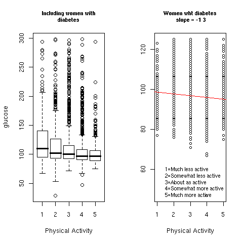
> par(mfrow=c(1,2))
> plot(glucose~physactf,data=HERS)
> with(HERS[HERS\$diabetes==0,], stripchart(glucose~physactf,vertical=T,cex=.8,pch=1))
> abline(HERS.lm1 <- lm(glucose~physact,data=HERS,subset=diabetes==0),col="red")
Figure 2: Glucose level and Physical activity.
The overall F test might be obtained from the ANOVA table as well.
> anova(HERS.lm)
Analysis of Variance Table

Response: glucose
            Df Sum Sq Mean Sq F value   Pr(>F)
physactf     4   1673     418   4.431 0.001441 **
Residuals 2027 191345      94
---
Signif. codes:  0 *** 0.001 ** 0.01 * 0.05 . 0.1   1
The design matrix can be obtained with model.matrix; in our case, this will
be a 2032 by 5 matrix and here is a truncated output:
> head(model.matrix(HERS.lm))
  (Intercept) physactf2 physactf3 physactf4 physactf5
1           1         0         0         0         1
2           1         0         0         0         0
4           1         0         0         0         0
5           1         1         0         0         0
6           1         0         1         0         0
8           1         0         0         0         1
If we remove the intercept but include the same 5 levels factor physactf, we
will obviously get diffent results than what was obtained with the preceding
model.
> HERS.lm2 <- lm(glucose~-1+physactf,data=HERS,subset=diabetes==0)
> summary(HERS.lm2)
Call:
lm(formula = glucose ~ -1 + physactf, data = HERS, subset = diabetes ==
    0)

Residuals:
     Min       1Q   Median       3Q      Max
-48.9867  -6.9867  -0.9867   5.8056  29.8571

Coefficients:
          Estimate Std. Error t value Pr(>|t|)
physactf1  98.4206     0.9393   104.8   <2e-16 ***
physactf2  97.5621     0.5414   180.2   <2e-16 ***
physactf3  97.1944     0.3742   259.7   <2e-16 ***
physactf4  95.9867     0.3734   257.1   <2e-16 ***
physactf5  95.1429     0.6120   155.5   <2e-16 ***
---
Signif. codes:  0 *** 0.001 ** 0.01 * 0.05 . 0.1   1

Residual standard error: 9.716 on 2027 degrees of freedom
Multiple R-squared:  0.99,     Adjusted R-squared:  0.99
F-statistic: 4.023e+04 on 5 and 2027 DF,  p-value: < 2.2e-16
At present, each `beta`i represents an estimate of the mean response in
the ith category, and the design matrix now looks like
> head(model.matrix(HERS.lm2))
  physactf1 physactf2 physactf3 physactf4 physactf5
1         0         0         0         0         1
2         1         0         0         0         0
4         1         0         0         0         0
5         0         1         0         0         0
6         0         0         1         0         0
8         0         0         0         0         1
However, t-test and global F-test are not relevant anymore since they are
based on a comparison to a zero baseline (check the t-value greater than 100,
for example). On the contrary, we are much more interested in between-groups
comparisons, taking group 1 as the reference group (“much less active”
condition) since it is the most relevant for the purpose of the study
(variation of glucose level with intensity of daily activities). An
alternative strategy would be to use a multiple comparison approach, like the
Dunnett procedure [a], to compare each group to the control one.
Consider the following situation: We have 5 groups who were enrolled in a
randomized clinical trial. Four of them have been administered different doses
of a pharmaceutical preparation (whatever the effect we might be
measuring). Group 1 will be the reference group (placebo), while groups 2 to 5
will be the experimental groups. Only group 5 is suspected to have a lowered
mean response rate.
> ni <- 20
> x <- gl(5,ni)
> y <- c(rnorm(ni,10,2),replicate(3,rnorm(ni,12,2)),rnorm(ni,6,2.5))
> xy <- data.frame(x=x,y=y)
> summary(xy)
 x            y
 1:20   Min.   : 0.6874
 2:20   1st Qu.: 8.9039
 3:20   Median :10.9522
 4:20   Mean   :10.2007
 5:20   3rd Qu.:12.3148
        Max.   :17.1221
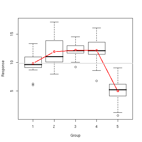
> boxplot(y~x,xlab="Group",ylab="Response")
> lines(1:5,tapply(y,x,mean),type="b",col="red",lwd=2)
> abline(h=mean(y[x==1]),col="lightgray",lwd=2)
Results are presented in [Fig. 3].
Figure 3: Response distribution and mean profiles in the simulated drug experiment.
Now, let's look at a simple comparison between Group 1 and Group 2:
> xy.lm <- lm(y~x,xy)
> library(contrast)
> contrast(xy.lm,list(x='1'),list(x='2'))
lm model parameter contrast

   Contrast      S.E.     Lower     Upper     t df Pr(>|t|)
1 -2.051397 0.6360268 -3.314069 -0.788724 -3.23 95   0.0017
The contrast function allows to test for any linear contrast. The help
function provides the following information:
contrast.lm             package:contrast             R Documentation

General Contrasts of Regression Coefficients

Description:

     This function computes one or more contrasts of the estimated
     regression coefficients in a fit from one of the functions in
     Design, along with standard errors, confidence limits, t or Z
     statistics, P-values.

Usage:

     contrast(fit, ...)
     ## S3 method for class 'lm':
     contrast(fit, ...)
     ## S3 method for class 'gls':
     contrast(fit, ...)
     ## S3 method for class 'lme':
     contrast(fit, ...)
     ## S3 method for class 'geese':
     contrast(fit, ...)
The complete
documentation can be found on R CRAN. There is also an
R
vignette which describes the detailed implementation of contrasts for linear
models.
“Unfortunately”, it provides Wald test and not F test as some other
statistical packages, like Statistica or SPSS [b], do propose.

|
About contrast coding within R
There are many routes to contrast coding with R. Among the classical way, one
can set up the contrast by hand, using contrast vector or matrix notation. For
example, we can build a contrast like (1,1,-1,-1) aiming at comparing two
conditions with two other conditions by issuing
> C <- c(1,1,-1,-1)
> aov(cbind(x11,x12,x21,x22) %*% C ~ group, data)
(but see the excellent
tutorial written by
Baron and Li).
As an alternative, one can specify default contrast coding, such as
> options(contrasts = c("contr.helmert", "contr.poly"))
in the R shell. This would apply to all formula-based models (lm, aov,
lme, etc.) that make use of such contrasts.
There is also a function that facilitate contrast coding (see
?contrasts). Furthermore, the MBESS package also provides several
functions for multiple comparisons, as well as the car package. Finally, the
Design package is entirely devoted to linear modelling, and the contrast
package used above relies on it. To get an idea, just check the R online help:
> help.search("contrast")
|
Using a standard t-test (t.test(y[x==1],y[x==2],var.equal=TRUE)) is
obviously not a good idea since it doesn't consider the right residual SS.
For the F test, it happen to be very easy once we recall that such statistics
is calculated as the ratio between SS for the differences and residual SS.
The same result can be obtained by checking the output of the corresponding
regression coefficients since x is here considered as a categorical
variable. We can see in the following listing that the t value for x2 equals
3.225, with p=0.0017.
> summary(xy.lm)
Call:
lm(formula = y ~ x, data = xy)

Residuals:
    Min      1Q  Median      3Q     Max
-5.3143 -0.9061 -0.1659  1.1268  5.2257

Coefficients:
            Estimate Std. Error t value Pr(>|t|)
(Intercept)   9.8450     0.4497  21.891  < 2e-16 ***
x2            2.0514     0.6360   3.225 0.001726 **
x3            2.3090     0.6360   3.630 0.000458 ***
x4            2.2583     0.6360   3.551 0.000600 ***
x5           -4.8403     0.6360  -7.610 1.98e-11 ***
---
Signif. codes:  0 '***' 0.001 '**' 0.01 '*' 0.05 '.' 0.1 ' ' 1

Residual standard error: 2.011 on 95 degrees of freedom
Multiple R-Squared: 0.6608,     Adjusted R-squared: 0.6465
F-statistic: 46.27 on 4 and 95 DF,  p-value: < 2.2e-16
We propose to use a simulation study to compare the two approaches (regression
vs. ANOVA or t-test). We thus need to define a sample of observations whose
values might vary according to the level of an exogenous factor.
Let's start with a two groups experiment. We assume that yi residuals follow
a normal distribution, and a model like
in the ANOVA notation, or, equivalently,
using the regression modelling notation.
> n <- 100
> x <- gl(2,n/2,n,labels=0:1)
> y <- c(rnorm(n/2,25,3),rnorm(n/2,30,2.5))
> tapply(y,x,mean)
       0        1
25.10533 29.95281
> tapply(y,x,var)
       0        1
7.848420 4.981874
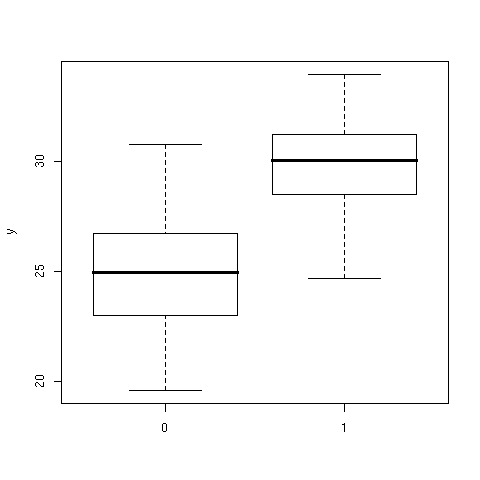
> plot(x,y)
As can be seen, there is quite the same within-group variability (though we
specify a lesser sd when drawing the second sample) while we observe a 5
points (approx.) difference between the groups. The data are summarized with
the help of box-and-whiskers charts in [Fig. 4].
Figure 4: Boxplots of the y response for the two groups.
A simple linear regression gives
> y.lm <- lm(y~x)
> summary(y.lm)
Call:
lm(formula = y ~ x)

Residuals:
    Min      1Q  Median      3Q     Max
-5.5379 -1.5516 -0.1123  1.5510  5.6804

Coefficients:
            Estimate Std. Error t value Pr(>|t|)
(Intercept)  25.1053     0.3582  70.089  < 2e-16 ***
x1            4.8475     0.5066   9.569 1.04e-15 ***
---
Signif. codes:  0 '***' 0.001 '**' 0.01 '*' 0.05 '.' 0.1 ' ' 1

Residual standard error: 2.533 on 98 degrees of freedom
Multiple R-Squared: 0.483,      Adjusted R-squared: 0.4778
F-statistic: 91.57 on 1 and 98 DF,  p-value: 1.042e-15
and the results is highly significant, if we focus on the slope
estimate. Here, x is treated as a categorical variable but the same results
would have been obtained if it was first converted to a numerical one (see
Problem 4.1).
Now, what gives a t-test (for independent samples), assuming homoscedasticity?
> t.test(y~x,var.equal=TRUE)
        Two Sample t-test

data:  y by x
t = -9.5694, df = 98, p-value = 1.042e-15
alternative hypothesis: true difference in means is not equal to 0
95 percent confidence interval:
 -5.852736 -3.842221
sample estimates:
mean in group 0 mean in group 1
       25.10533        29.95281
We get exactly the same result, except for the sign of the t statistics. The
result is highly significant, which is not very surprising given the sample
size we used and the effect size we choose (+5 points between the two groups).
Now, if we extend this simulation to a three groups design, we can check that
we will get exactly the same pattern of results, whether we look at the output
of regression model or of an ANOVA table.
> x <- gl(3,n/3,n,labels=0:2)
> y <- as.numeric(x) + rnorm(n)
> by(y,x,summary)
INDICES: 0
   Min. 1st Qu.  Median    Mean 3rd Qu.    Max.
-0.6392  0.1236  0.8728  0.8005  1.2560  2.1900

INDICES: 1
   Min. 1st Qu.  Median    Mean 3rd Qu.    Max.
-0.6749  1.1830  1.6820  1.6710  2.1510  3.8590

INDICES: 2
   Min. 1st Qu.  Median    Mean 3rd Qu.    Max.
  1.215   2.291   2.880   2.955   3.521   5.104
> plot(x,y)
> stripchart(y~x,vertical=T)
> points(1:3,tapply(y,x,mean),pch="x",cex=2,col="red")
> abline(lm(y~as.numeric(x)),col="red")
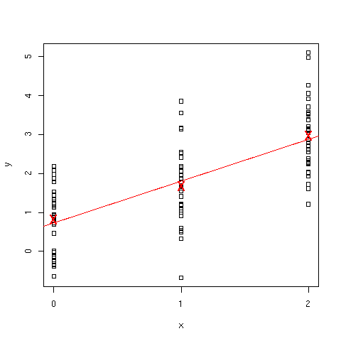
Evolution of y between the three groups is illustrated in [Fig. 5] (boxplots
issued by the plot(x,y) command have been discarded). Straight line
represents the regression line, and group means are represented as red
crosses.
Figure 5: Evolution of y as a function of factor level.
Regression output (see below) indicates that y values differ according to
factor level as each coefficient appears highly significant.
> summary(lm(y~x))
Call:
lm(formula = y ~ x)

Residuals:
     Min       1Q   Median       3Q      Max
-2.34550 -0.63749  0.03854  0.48981  2.18849

Coefficients:
            Estimate Std. Error t value Pr(>|t|)
(Intercept)   0.8005     0.1509   5.304 7.15e-07 ***
x1            0.8701     0.2151   4.045 0.000105 ***
x2            2.1542     0.2151  10.016  < 2e-16 ***
---
Signif. codes:  0 '***' 0.001 '**' 0.01 '*' 0.05 '.' 0.1 ' ' 1

Residual standard error: 0.8801 on 97 degrees of freedom
Multiple R-Squared: 0.511,      Adjusted R-squared: 0.5009
F-statistic: 50.68 on 2 and 97 DF,  p-value: 8.534e-16
In this case, each mean is compared with baseline level (the group coded
0). The first coefficient estimate, x1, is thus estimated as the difference
between group 1 and group 0.
> mean(y[x==1])-mean(y[x==0])
[1] 0.8700501
If we use an ANOVA, we also get significant result for the factor X. But,
now, the interpretation is less detailed and we only have the MS of X compared
to residual MS.
> summary(aov(y~x))
            Df Sum Sq Mean Sq F value    Pr(>F)
x            2 78.522  39.261  50.684 8.534e-16 ***
Residuals   97 75.139   0.775
---
Signif. codes:  0 '***' 0.001 '**' 0.01 '*' 0.05 '.' 0.1 ' ' 1
Assessing between-groups comparison would imply to use orthogonal contrast,
for instance treatment contrast (see the previous note).
However, we will get the same output than with the lm function by using
summary.lm instead of just summary on aov object:
> summary.lm(aov(y~x))
Call:
aov(formula = y ~ x)

Residuals:
     Min       1Q   Median       3Q      Max
-2.34550 -0.63749  0.03854  0.48981  2.18849

Coefficients:
            Estimate Std. Error t value Pr(>|t|)
(Intercept)   0.8005     0.1509   5.304 7.15e-07 ***
x1            0.8701     0.2151   4.045 0.000105 ***
x2            2.1542     0.2151  10.016  < 2e-16 ***
---
Signif. codes:  0 '***' 0.001 '**' 0.01 '*' 0.05 '.' 0.1 ' ' 1

Residual standard error: 0.8801 on 97 degrees of freedom
Multiple R-Squared: 0.511,      Adjusted R-squared: 0.5009
F-statistic: 50.68 on 2 and 97 DF,  p-value: 8.534e-16
Indeed, without any other covariates, ANOVA and regression on categorical
variable always lead to the same results.
> model.tables(aov(y~x))
Tables of effects

 x
         0       1      2
    -0.998 -0.1280  1.156
rep 34.000 33.0000 33.000
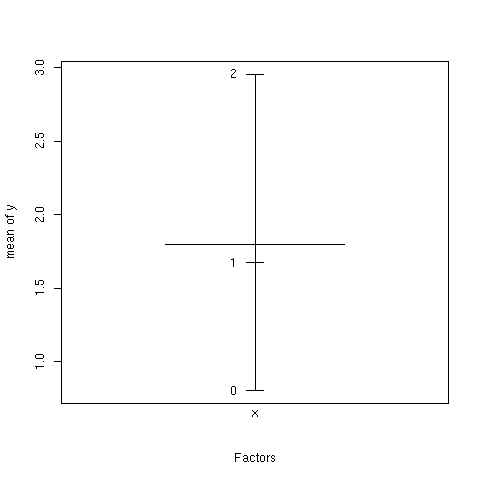
> plot.design(y~x)
Figure 6: Group means difference.
