First, we refit the model to get all of the information. In this
model, age is treated as a categorical variable, with 5 levels, namely
]39,40], ]40,45], ]45,50], ]50,55], ]55,59].
The youngest age group is taken as the reference category.
> WCGS <- read.table("wcgs.txt",header=TRUE,sep="\t")
> table(WCGS\$chd69,WCGS\$agec)

              0    1    2    3    4
  Noncases  512 1036  680  463  206
  Cases      31   55   70   65   36
> WCGS\$agec <- as.factor(WCGS\$agec)
> WCGS.glm3 <- glm(chd69~agec,data=WCGS,family=binomial())
> summary(WCGS.glm3)

Call:
glm(formula = chd69 ~ as.factor(agec), family = binomial(), data = WCGS)

Deviance Residuals:
    Min       1Q   Median       3Q      Max
-0.5676  -0.4427  -0.3429  -0.3216   2.4444

Coefficients:
            Estimate Std. Error z value Pr(>|z|)
(Intercept)  -2.8043     0.1850 -15.162  < 2e-16 ***
agec1        -0.1315     0.2310  -0.569 0.569298
agec2         0.5307     0.2235   2.374 0.017580 *
agec3         0.8410     0.2275   3.697 0.000218 ***
agec4         1.0600     0.2585   4.100 4.13e-05 ***
---
Signif. codes:  0 '***' 0.001 '**' 0.01 '*' 0.05 '.' 0.1 ' ' 1

(Dispersion parameter for binomial family taken to be 1)

    Null deviance: 1781.2  on 3153  degrees of freedom
Residual deviance: 1736.3  on 3149  degrees of freedom
AIC: 1746.3

Number of Fisher Scoring iterations: 5
The required computation can be done manually or with
R. Exponentiation of the regression coefficient for the third age
group gives the odds ratio associated with CHD Risk for individuals
aged between 45 and 50 and individuals ages 40 years old or less. What
we want is the fourth vs. the third category of age. It can easily be
shown that the corresponding log odds equals
that is 1.060-0.841=0.219. Exponentiating the result, we get an OR of
1.245. There is an 25% increase in the coronary disease risk for
person aged five to ten years old.
Using R, we reach the same conclusion, as shown in the following code.
> exp(coef(WCGS.glm3)[5]-coef(WCGS.glm3)[4])
   agec4
1.244810
Another solution is to refit the model using the third age group as the
reference catgeory. This would obviously not make sense to interpret
the regression coefficient with respect to this reference value, but,
anyway, this gives the expected result.
> agec2 <- relevel(WCGS\$agec,'3')
> levels(agec2)
[1] "3" "0" "1" "2" "4"
> WCGS.glm3b <- glm(chd69~agec2,data=WCGS,family=binomial())
> summary(WCGS.glm3b)
Call:
glm(formula = chd69 ~ agec2, family = binomial(), data = WCGS)

Deviance Residuals:
    Min       1Q   Median       3Q      Max
-0.5676  -0.4427  -0.3429  -0.3216   2.4444

Coefficients:
            Estimate Std. Error z value Pr(>|z|)
(Intercept)  -1.9633     0.1325 -14.823  < 2e-16 ***
agec20       -0.8410     0.2275  -3.697 0.000218 ***
agec21       -0.9724     0.1915  -5.077 3.84e-07 ***
agec22       -0.3103     0.1825  -1.700 0.089096 .
agec24        0.2190     0.2240   0.978 0.328275
---
Signif. codes:  0 '***' 0.001 '**' 0.01 '*' 0.05 '.' 0.1 ' ' 1

(Dispersion parameter for binomial family taken to be 1)

    Null deviance: 1781.2  on 3153  degrees of freedom
Residual deviance: 1736.3  on 3149  degrees of freedom
AIC: 1746.3

Number of Fisher Scoring iterations: 5
Though the calculations might be handled quite in a similar fashion as
above, we will use R directly. We already compared 55-year-old
individuals with and without arcus. The estimated odds ratio was 1.01
([0.68—1.51]), thus we conclude to the absence of difference of risk
for people of the same age (the prevalence being very low, we are
allowed to interpret OR as RR). Now, contrasting 40 vs. 55-year-old
people gives a different picture.
> library(Design)
> WCGS.glm11bis <- lrm(chd69~age*arcus,data=WCGS)
> cc <- contrast(WCGS.glm11bis,list(age=55,arcus='Exposed'),
                   list(age=40,arcus='Exposed'))
> exp(unlist(cc[2:5]))
Contrast.1         SE    Lower.1    Upper.1
  1.817128   1.309514   1.071159   3.082600
The estimated OR is 1.82 with a 95% confidence interval of
[1.07—3.08]. There is an 82% increase in risk when people are 15
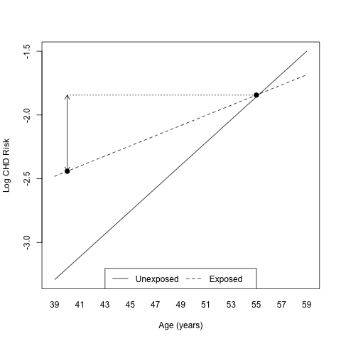
years older compared to people aged 40. In the figure reproduced from
the book below (Fig. 6.2), it is clear that the risk is even
more pronounced for individual with arcus than those unexposed to this
risk factor. Graphically, we'll reach the same conclusion about
increase of risk between 40 and 55 years for exposed individuals. The
difference in log odds for the two points highlighted on [Fig. 1] is
0.598, and taking the exponential gives an OR of 1.817.
Figure 1: Log odds of CHD and Age for individuals with and without Arcus Senilis.
The Hosmer-Lemeshow test [2] [pp. 149—170] relies on the evaluation
of the “concordance” between observed and expected frequencies under
the logistic model. To do this comparison, groups of ordered estimated
outcome probabilities are constituted, usually ten equal-size groups
based on deciles of the probability distribution). The underlying
(null) hypothesis is that both frequencies distribution agree, and it
can be tested using a `chi`2 with k-2 degrees of freedom, where
k is the number of groups. Exemples of the use of this statistics can
be found in e.g. [3] or [4].
Note that this test suffers from low power (Vittinghoff et al.,
p. 194), and as proposed by F. Harrell [1], we'll be using
residuals.lrm() as a better GoF test. But let's see how the HL test
works.
The expanded logistic model for CHD Events (Table 6.17) was obtained
as follows:
> WCGS.glm13 <- glm(y~age_10+chol_50+sbp_50+bmi_10+smoke+dibpat
                    +bmi_10:chol_50+bmi_10:sbp_50,
                    data=WCGS,family=binomial())
> summary(WCGS.glm13)

Call:
glm(formula = chd69 ~ age_10 + chol_50 + sbp_50 + bmi_10 + smoke +
    dibpat + bmi_10:chol_50 + bmi_10:sbp_50, family = binomial(),
    data = WCGS)

Deviance Residuals:
    Min       1Q   Median       3Q      Max
-1.1970  -0.4477  -0.3148  -0.2138   2.9126

Coefficients:
               Estimate Std. Error z value Pr(>|z|)
(Intercept)    -3.41143    0.15019 -22.714  < 2e-16 ***
age_10          0.59150    0.12002   4.929 8.29e-07 ***
chol_50         0.59489    0.07665   7.761 8.40e-15 ***
sbp_50          1.00917    0.20651   4.887 1.02e-06 ***
bmi_10          1.01021    0.30093   3.357 0.000788 ***
smoke           0.59479    0.14068   4.228 2.36e-05 ***
dibpat          0.72215    0.14487   4.985 6.20e-07 ***
chol_50:bmi_10 -0.69208    0.24392  -2.837 0.004550 **
sbp_50:bmi_10  -1.39568    0.62806  -2.222 0.026269 *
---
Signif. codes:  0 '***' 0.001 '**' 0.01 '*' 0.05 '.' 0.1 ' ' 1

(Dispersion parameter for binomial family taken to be 1)

    Null deviance: 1779.2  on 3141  degrees of freedom
Residual deviance: 1578.6  on 3133  degrees of freedom
  (12 observations deleted due to missingness)
AIC: 1596.6

Number of Fisher Scoring iterations: 6
We need to create a matrix including both the expected and observed
frequencies. The former are obtained using predict(). We already
computed them when we studied the ROC curve.
> WCGS.glm13.predAll <- predict(WCGS.glm13,type="response")
> tmp <- cbind(predicted=WCGS.glm13.predAll,
               observed=WCGS$chd69[as.numeric(names(WCGS.glm13.predAll))])
The next steps involve computing the aggregated frequencies.
> k <- 10
> (grp <- quantile(tmp[,1],seq(0,1,length=k)))
         0%   11.11111%   22.22222%   33.33333%   44.44444%   55.55556%
0.001022747 0.016941975 0.026733528 0.037837667 0.050264964 0.065064656
  66.66667%   77.77778%   88.88889%        100%
0.087515979 0.118360364 0.172746778 0.586610935
> lb <- cut(tmp[,1],breaks=as.numeric(grp),labels=FALSE,ordered_result=TRUE)
> table(lb)
lb
  1   2   3   4   5   6   7   8   9
349 349 349 349 349 349 349 349 349
We expect 10% of observations falling between 0.001 and 0.017, but
only 10% are expected to lie between 0.173 and 0.587, confirming the
observation that CHD is a relatively rare event.
However, it seems that this model performs relatively poorly in terms
of prediction because we predict only 5 cases out of 2142 while there
are in fact 257 cases in the original data.
> table(fit=ifelse(tmp[,1]>0.5,1,0),obs=tmp[,2]-1)
   obs
fit    0    1
  0 2883  254
  1    2    3
In essence, this confirms the ROC analysis as well as the
specification tests used pp. 192—193 of Vittinghoff et al.
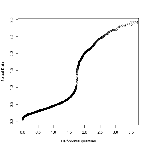
Another way to look at potential outliers is to use something like an
Q-Q plot but more oriented toward GLM data. This is what proposed
J. Faraway [5] using the halfnorm() function, see
[Fig. 2]. Details about construction of this kind of plot are given
pp. 129—130.
Figure 2: Half-normal plot of the studentized residuals for the expanded Logistic Model.

|
GoF tests for the Rasch Model
In educational assessment, the
Rasch Model (aka,
one-parameter logistic model) is widely used to calibrate items and
deliver standardized test scores. Items that do not fit the Rasch
Model are most of the time removed from the questionnaire or test
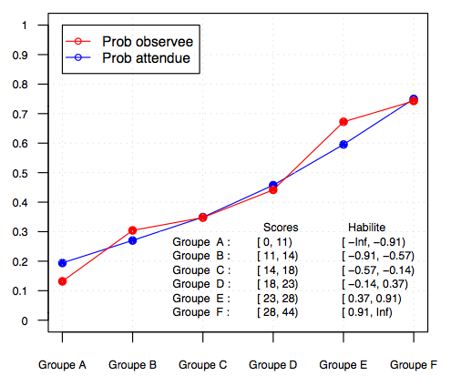
battery in order not to alter the measurement scale. When items
parameters (in such a context, they are called the difficulties of
the items) have been estimated, one way to check for model adequacy
consists in graphically examining the concordance between observed and
expected frequencies of a correct answer to a given item. Such a plot
is provided below.
Additional informations can be get from:
The gOfIRT() function in the eRm package proposes various GoF for
IRT Models, including Hosmer-Lemeshow test.
|
Now, using F. Harrell's package, we raise similar conclusions.
> library(Design)
> ?residuals.lrm
The on-line help provides further indication on the kind of GoF test
that are currently implemented in the Design package.
     For a binary logistic model fit, computes the following residuals,
     letting P denote the predicted probability of the higher category
     of Y, X denote the design matrix (with a column of 1s for the
     intercept), and L denote the logit or linear predictors: ordinary
     (Y-P), score (X (Y-P)), pearson ((Y-P)/sqrt{P(1-P)}), deviance
     (for Y=0 is -sqrt{2|log(1-P)|}, for Y=1 is sqrt{2|log(P)|}, pseudo
     dependent variable used in influence statistics  (L +
     (Y-P)/(P(1-P))), and partial (X_{i}beta_{i} + (Y-P)/(P(1-P))).

     Will compute all these residuals for an ordinal logistic model,
     using as temporary binary responses dichotomizations of Y, along
     with the corresponding P, the probability that Y >=q cutoff.  For
     'type="partial"', all  possible dichotomizations are used, and for
     'type="score"', the actual components of the first derivative of
     the log likelihood are used for an ordinal model.  Alternatively,
     specify 'type="score.binary"' to use binary model score residuals
     but for all cutpoints of Y (plotted only, not returned). The
     'score.binary',  'partial', and perhaps 'score' residuals are
     useful for checking the proportional odds assumption. If the
     option 'pl=TRUE' is used to plot the 'score' or 'score.binary'
     residuals,  a score residual plot is made for each column of the
     design (predictor) matrix, with 'Y' cutoffs on the x-axis and the
     mean +- 1.96 standard errors of the score residuals on the y-axis.
      You can instead use a box plot to display these residuals, for
     both 'score.binary' and 'score'. Proportional odds dictates a
     horizontal 'score.binary' plot.  Partial residual plots use smooth
     nonparametric estimates, separately for each cutoff of Y.  One
     examines that plot for parallelism of the curves to check the
     proportional odds assumption, as well as to see if the predictor
     behaves linearly.

     Also computes a variety of influence statistics and the  le Cessie
     - van Houwelingen - Copas - Hosmer unweighted sum of squares test
     for global goodness of fit, done separately for each cutoff of Y
     in the case of an ordinal model.

     The 'plot.lrm.partial' function computes partial residuals for a
     series of binary logistic model fits that all used the same
     predictors and that specified 'x=TRUE, y=TRUE'.  It then computes
     smoothed partial residual relationships (using 'lowess' with
     'iter=0') and plots them separately for each predictor, with
     residual plots from all model fits shown on the same plot for that
     predictor.
There is also a complete discussion of GLM diagnostic in [5]
(Chapter 6, pp. 123—135).
Basically, the scheme for expanding the odds ratio formula can be best
understood if we consider the Table below, where E stands for
exposition to risk factor (E+ = exposed, E- = non exposed) and M for
the disease (e.g. M+ = dead, M- = alive).
The odds of being dead while a subject has been exposed is given by
a/b, while that of being alive while exposed is c/d. Thus, the
odds ratio is computed as
In the above formula, we have conditioned the outcome on the risk
factor. It can easily be shown that reversing the conditionning factor
leads to the same results, which is a property of the odds ratio
only. Indeed, we get (a/c)/(b/d) = ad/bc. It doesn't hold for relative
risk for instance, because it make sense only when we condition on the
risk factor; in this case, it happens to be [a/(a+b)]/[c/(c+d)]. There
are other reasons that makes life easier when working with odds ratio:
first, they are directly derivend from the regression coefficients of
the logistic regression; second, they have asymptotic distribution
that allow to derive reliable confidence intervals. However, we must
ackonwledge the fact that their interpretation is less easy than
relative risk, which is why most of the time we found an
interpretation of empirical results based on RR. It should be noted
that when the prevalence of the disease under consideration is low (<
10%), both values are convergent.
This problem refers to a Complementary Log-Log regression model
applied to a CDC transmission study. Data are not available, but we
could simulate a small dataset to illustrate this king of GLM.


