Bayesian analysis with R
I am just reading Data Analysis Using Regression and Multilevel/Hierarchical Models from Andrew Gelman and Jennifer Hill (Cambridge University Press, 6th printing 2008). The companion website includes all data sets and R code. Another useful reference for R users is Bayesian Computation with R in the Springer’s UseR series, from J. ALbert.
First of all, I found that graphical displays are overall very nicely drawn on the B&W version of the book. For instance, the two plots below include all information I ever wanted to see from a logistic regression (here, exported at 300 DPI for better viewing).


Chapters 9, 10, and 23 provide important discussions and illustrations regarding causal inference, and are well-suited for biomedical studies (e.g., what variables shall we control for in pre- and post-treatment studies). There are also interesting illustration with IRT in Chapter 14.
A. Gelman makes extensive use of BUGS for bayesian computation, but BUGS software doesn’t work on Mac OS X. With the newly released version of JAGS 2.1.0 (as of May, the 12th), it must, however, be possible to do most of the computation shown in Gelman’s book. The corresponding R packages are called rjags and R2jags, the latter being developed by one of Gelman’s student, Yu-Sung Su.
JAGS stands for “Just Another Gibbs Sampler” and is a tool for analysis of Bayesian hierarchical models using Markov Chain Monte Carlo (MCMC) simulation, but see M. Plummer’s main article.1 In R2jags, the rjags() function ensures the main part of the computation and need a proper BUGS model stored in a text file. In what follows, we will restrict ourselves on the original rjags package.
For the sake of illustration, we will consider the following example from Broemeling’s book, Bayesian Biostatistics and Diagnostic Medicine (Chapman & Hall/CRC, 2007). It is a meta-analysis on 22 RCTs of beta-blockers to prevent mortality after myocardial infarction, which is available in WinBUGS example data set.2 An example of the available data is shown in the following table.
| Trial | Treated | Control |
| 1 | 3/38 | 3/39 |
| 2 | 7/114 | 14/116 |
| 3 | 5/69 | 11/93 |
| 4 | 102/1533 | 127/1520 |
| ••• | ••• | ••• |
| 20 | 32/209 | 40/218 |
| 21 | 27/391 | 43/364 |
| 22 | 22/680 | 39/674 |
The corresponding BUGS model reads as follows:
model {
   for (i in 1:Num) {
     rt[i] ~ dbin(pt[i], nt[i]);
     rc[i] ~ dbin(pc[i], nc[i]);
     logit(pc[i]) <- mu[i]
     logit(pt[i]) <- mu[i] + delta[i];
     delta[i] ~ dnorm(d, tau);
     mu[i] ~ dnorm(0.0, 1.0E-5);
   }
   d ~ dnorm(0.0, 1.0E-6);
   tau ~ dgamma(1.0E-3, 1.0E-3);
   delta.new ~ dnorm(d,tau);
   sigma <- 1/sqrt(tau);
}
Here, each trial is modeled with a different probability of success for the control and treated patients, and the binomial probabilities are expressed on the logit scale with a differential, d[i], between the two groups. This difference is assumed to follow a gaussian with parameters delta and tau, drawn from an $\mathcal{N}(0,10^6)$ and a $\text{Gamma}(0.001,0.001)$, respectively. All $\mu$ and $\delta$ are initialized to 0.
The R code is rather simple:
m <- jags.model("blocker.bug", data, list(inits,inits), 2)
update(m, 3000)
x <- coda.samples(m, c("d","delta.new","sigma"), n.iter=30000, thin=10)
plot(x)
apply(x[[1]], 2, summary)
where blocker.bug is simply the model in BUGS syntax, data is a list with the 22 rc, nc, rt, and nt values. In the inits list, all is set to 0 except tau which is given a value of 1.
This took about 20 sec. to complete on my Mac (Core 2 Duo, 2.8 GHz) and the MCMC results are summarized below (thanks to the coda package).
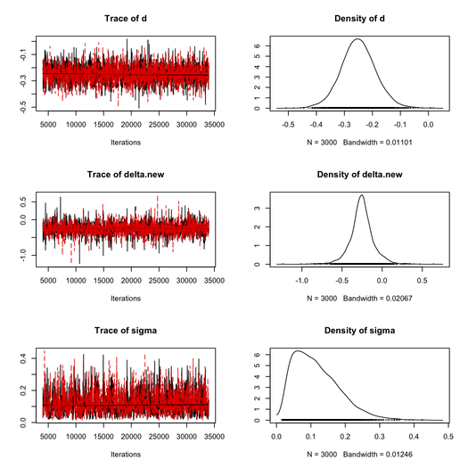
For the first chain, we get as posterior estimates:
| Parameter | Mean | SD | 1st Qu. | Median | 3rd Qu. |
| δ | -0.2523 | 0.1481 | -0.3239 | -0.2564 | -0.1810 |
| σ | 0.1040 | 0.0668 | 0.0617 | 0.1040 | 0.1560 |
This is close to values reported in Broemeling although they use a different setting with 50,000 draws from the posterior distribution of $\delta$ and $\sigma=1/\tau$.
There are other diagnostic plots useful for assessing chains convergence, including gelman.plot(), crosscorr.plot(). For assessing goodness of fit or comparing two models, the deviance information criterion (DIC) can be calculated with dic.samples. But I think I will definitively deserve this to another post.