Multiple comparisons and p-value adjustment
Some time ago, I wrote a tutorial on various procedures applied in a multiple comparisons framework, “Comparaisons multiples”. It’s in French and includes R source code: pdf tutorial, R code, htmlized R code. Now, I feel it’s time to update a little bit these old notes with new material. This is motivated by my new interest toward bioinformatics and medical imaging that are both facing the n p and p-value correction problems.
Multiple comparisons arise when one wants to compare more than two things at the same time (i.e. for the same dataset, in the same explanatory framework). Why do we have to adapt the usual test statistics? Because these multiple tests (of hypothesis) are generally not carried out in an independent way, thus leading to an inflation of the overall type I error rate. In other words, when faced with say 10 comparisons on the same data, the probability of falsely detecting a significant difference becomes greater than the classical 5% level. For a general introduction to multiple comparison procedure, the reader may be interested in sup(6)/sup. Other references are (5,7) and (8) (especially, Chapter 5) but the latter two are a bit more tricky.
Actually, there are two main packages that can handle multiple comparison, both relying on a different view of the type I error:
multcomp(R vignette), for “Simultaneous tests and confidence intervals for general linear hypotheses in parametric models, including linear, generalized linear, linear mixed effects, and survival models.”multtest(see Dudoit and van der Laan,(7) and a series of talks here: 1, 2, 3), for “Non-parametric bootstrap and permutation resampling-based multiple testing procedures for controlling the family-wise error rate (FWER), generalized family-wise error rate (gFWER), tail probability of the proportion of false positives (TPPFP), and false discovery rate (FDR). Single-step and step-wise methods are implemented. Tests based on a variety of t- and F-statistics (including t-statistics based on regression parameters from linear and survival models) are included. Results are reported in terms of adjusted p-values, confidence regions and test statistic cutoffs. The procedures are directly applicable to identifying differentially expressed genes in DNA microarray experiments.”
Interestingly, the former is attached to the Social Sciences Task View while the latter is on Bioconductor.
Also, I should mention the Design (see its contrast() function) package by F. Harrell, the npmc package for non parametric multiple comparisons, but see R Site Search, with keyword = “multiple comparison”.
For the purpose of the illustration, we will use the data from the Cholesterol study (included in the multcomp package):
A clinical study was conducted to assess the effect of three formulations of the same drug on reducing cholesterol. The formulations were 20mg at once (
1time), 10mg twice a day (2times), and 5mg four times a day (5times). In addition, two competing drugs were used as control group (drugDanddrugE). The purpose of the study was to find which of the formulations, if any, is efficacious and how these formulations compare with the existing drugs.
Using multcomp
The main function is called glht() and its description indicates that it provides general linear hypotheses and multiple comparisons for parametric models, including generalized linear models, linear mixed effects models, and survival models. Well, it covers quite interesting models for a biostatistician.
First, let’s try a basic ANOVA model on the “choslesterol” data.
library(multcomp)
data(cholesterol)
lm1 <- aov(response ~ trt, data=cholesterol)
summary(lm1)
This yields the following ANOVA table:
            Df  Sum Sq Mean Sq F value    Pr(>F)
trt          4 1351.37  337.84  32.433 9.819e-13 ***
Residuals   45  468.75   10.42
---
Signif. codes:  0 ‘***’ 0.001 ‘**’ 0.01 ‘*’ 0.05 ‘.’ 0.1 ‘ ’ 1
As can be seen from the resulting call to the aov() function (Recall that aov() is just a wrapper for the more general lm() function), the treatment main effect appears significant (the p-value is largely .001). This is not very surprising given the picture of the data shown in the figure below.
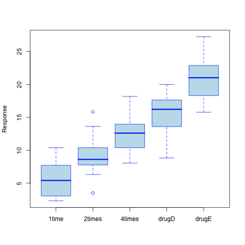
However, what can be said about the paired difference between consecutive formulations (20mg at once, 10mg twice a day, 5mg four times a day), and how do they compare to already in-use drugs (drugD and drugE)?
We may have a look at regression coefficient for each treatment, considering 1time as the baseline. This is done with summary.lm(lm1), and we get the results shown below:
Call:
aov(formula = response ~ trt, data = cholesterol)

Residuals:
      Min        1Q    Median        3Q       Max
-6.541770 -1.967203 -0.001575  1.890143  6.600830

Coefficients:
            Estimate Std. Error t value Pr(>|t|)
(Intercept)    5.782      1.021   5.665 9.78e-07 ***
trt2times      3.443      1.443   2.385   0.0213 *
trt4times      6.593      1.443   4.568 3.82e-05 ***
trtdrugD       9.579      1.443   6.637 3.53e-08 ***
trtdrugE      15.166      1.443  10.507 1.08e-13 ***
---
Signif. codes:  0 ‘***’ 0.001 ‘**’ 0.01 ‘*’ 0.05 ‘.’ 0.1 ‘ ’ 1

Residual standard error: 3.227 on 45 degrees of freedom
Multiple R-squared: 0.7425,	Adjusted R-squared: 0.7196
F-statistic: 32.43 on 4 and 45 DF,  p-value: 9.819e-13
This is quite informative but it just says that all treatment differ from the baseline which is usually not what we’re interested in. Here, the Intercept represents the mean response for 20mg at once:
with(cholesterol, mean(response[as.numeric(trt)==1]))
[1] 5.78197
We might be interested in which pairs of means (without consideration for the internal data structure, that is 3 different dosages + 2 classical drugs) are significatively different. This calls for something the Tukey HSD procedure which gives:
lm1.hsd <- TukeyHSD(lm1)
lm1.hsd
Results can be given both numerically,
  Tukey multiple comparisons of means
    95% family-wise confidence level

Fit: aov(formula = response ~ trt, data = cholesterol)

$trt
                  diff        lwr       upr     p adj
2times-1time   3.44300 -0.6582817  7.544282 0.1380949
4times-1time   6.59281  2.4915283 10.694092 0.0003542
drugD-1time    9.57920  5.4779183 13.680482 0.0000003
drugE-1time   15.16555 11.0642683 19.266832 0.0000000
4times-2times  3.14981 -0.9514717  7.251092 0.2050382
drugD-2times   6.13620  2.0349183 10.237482 0.0009611
drugE-2times  11.72255  7.6212683 15.823832 0.0000000
drugD-4times   2.98639 -1.1148917  7.087672 0.2512446
drugE-4times   8.57274  4.4714583 12.674022 0.0000037
drugE-drugD    5.58635  1.4850683  9.687632 0.0030633
or graphically,
opar <- par(mar=c(5,8,4,2),las=1)
plot(lm1.hsd)
abline(v=0,lty=2,col="gray50")
par(opar)
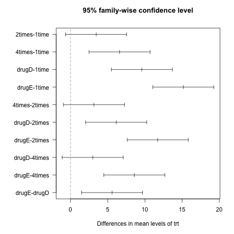
Now, we see that 7 pairs of difference of means out of 10 are different from 0 at the 5% level. Lower bound of 95% CI is always 1.
With the multcomp package, we have:
lm1.hsd2 <- glht(lm1, linfct = mcp(trt = "Tukey"))
summary(lm1.hsd2)
Simultaneous Tests for General Linear Hypotheses
Multiple Comparisons of Means: Tukey Contrasts
Fit: aov(formula = response ~ trt, data = cholesterol)
Linear Hypotheses:
Estimate Std. Error t value p value
2times - 1time == 0 3.443 1.443 2.385 0.138169
4times - 1time == 0 6.593 1.443 4.568 0.000352 ***
drugD - 1time == 0 9.579 1.443 6.637 < 1e-04 ***
drugE - 1time == 0 15.166 1.443 10.507 < 1e-04 ***
4times - 2times == 0 3.150 1.443 2.182 0.205103
drugD - 2times == 0 6.136 1.443 4.251 0.000993 ***
drugE - 2times == 0 11.723 1.443 8.122 < 1e-04 ***
drugD - 4times == 0 2.986 1.443 2.069 0.251209
drugE - 4times == 0 8.573 1.443 5.939 < 1e-04 ***
drugE - drugD == 0 5.586 1.443 3.870 0.003047 **
---
Signif. codes: 0 ‘***’ 0.001 ‘**’ 0.01 ‘*’ 0.05 ‘.’ 0.1 ‘ ’ 1
(Adjusted p values reported -- single-step method)
As can be seen, we obtain the same result. There is also a plot method that displays difference of means in a more convenient way (see ?plot.glht).
The main interface to glht() is the option linfct, which stands for linear function in the (G)LM framework. Any contrast can be passed directly (as a vector or matrix) to glht() or one can choose among those already constructed with the contrMat() function. Available contrasts coding are: Dunnett, Tukey, Sequen, AVE, Changepoint, Williams, Marcus, McDermott, UmbrellaWilliams, GrandMean. They all are referenced from Bretz et al.(4)
As for R default contrast coding scheme (i.e., treatment contrast), the default contrasts are Dunnett contrast, that is all k-1 comparisons are done with reference to the baseline, taken as the first level of the unordered factor.
As an illustration, let’s consider Dunnet contrast coding:
n <- c(10,20,30,40)
names(n) <- paste("dose", 1:4, sep="")
contrMat(n)
This yields:
Multiple Comparisons of Means: Dunnett Contrasts

group1 group2 group3 group4
group2 - group1     -1      1      0      0
group3 - group1     -1      0      1      0
group4 - group1     -1      0      0      1
> contrasts(as.factor(n))
   20 30 40
10  0  0  0
20  1  0  0
30  0  1  0
40  0  0  1
One would get a similar contrast matrix by calling contr.treatment(4). Note that such contrasts are not orthogonal to the Intercept and thus are not pure contrasts in standard LM Theory. Also note that some software doesn’t take the first level as the baseline, but instead choose the last one. It is the case for SAS at least. If we’re interested in getting the same result as SAS, we can either relevel the factor, specify which level to consider as the baseline (option base in contr.treatment(), or simply use the wrapper function contr.SAS().
The table below summarizes the different contrasts coding scheme in the multcomp package. Contrasts are expressed in rows and are labelled ci.
| Tukey | dose1 | dose2 | dose3 | dose4 |
|---|---|---|---|---|
| c1 | -1 | 1 | 0 | 0 |
| c2 | -1 | 0 | 1 | 0 |
| c3 | -1 | 0 | 0 | 1 |
| c4 | 0 | -1 | 1 | 0 |
| c5 | 0 | -1 | 0 | 1 |
| c6 | 0 | 0 | -1 | 1 |
All pairwise comparisons are allowed with Tukey contrasts. In contrast, for what are called Sequence (aka “Sequen”) contrasts we are “slicing” between consecutive pairwise treatment.
| Grand Mean | dose1 | dose2 | dose3 | dose4 |
|---|---|---|---|---|
| c1 | -1 | 1 | 0 | 0 |
| c2 | 0 | -1 | 1 | 0 |
| c3 | 0 | 0 | -1 | 1 |
Another class of useful contrasts is the Grand Mean model.
| Grand Mean | dose1 | dose2 | dose3 | dose4 |
|---|---|---|---|---|
| c1 | 0.9 | -0.2 | -0.3 | -0.4 |
| c2 | -0.1 | 0.8 | -0.3 | -0.4 |
| c3 | -0.1 | -0.2 | 0.7 | -0.4 |
| c4 | -0.1 | -0.2 | -0.3 | 0.6 |
Here, we take a different approach to the correction for Type I error rate inflation. As explained in Dudoit, S. and van der Laan (Section 2.8),(7) we only consider the control of Type I error under the true parameter values (or the true generating distribution, in the case of simulated data). Furthermore, this is not a strong control over the error rate (ER) as the proposed methodology doesn’t control the supremum of the Type I ER over parameter values satisfying all 2supM/sup possible subsets of null hypotheses.
The functions mt.rawp2adjp() and mt.plot() are by far the most useful routines for computing and displaying adjusted p-values. Let’s look at the example given in ?mt.rawp2adjp.
library(multtest)
data(golub)
smallgd <- golub[1:100,]
classlabel <- golub.cl
# Permutation unadjusted p-values and adjusted p-values for maxT procedure
res1 <- mt.maxT(smallgd,classlabel)
rawp <- res1$rawp[order(res1$index)]
# Permutation adjusted p-values for simple multiple testing procedures
procs <- c("Bonferroni","Holm","Hochberg","SidakSS","SidakSD","BH","BY")
res2 <- mt.rawp2adjp(rawp,procs)
To appreciate the differences between the different methods in a more convenient, we can plot the (sorted) adjusted p-values as a function of the number of rejected hypotheses. Again, following the on-line help, this can be done easily as follows:
allp <- cbind(res2$adjp[order(res2$index),],res1$adjp[order(res1$index)])
dimnames(allp)[[2]][9] <- "maxT"
procs <- dimnames(allp)[[2]]
procs[7:9] <- c("maxT","BH","BY")
allp <- allp[,procs]
cols <- c(1:4,"orange","brown","purple",5:6)
ltypes <- c(3,rep(1,6),rep(2,2))
# Ordered adjusted p-values
mt.plot(allp, teststat, plottype="pvsr", proc=procs, leg=c(80,0.4),
        lty=ltypes, col=cols, lwd=2)
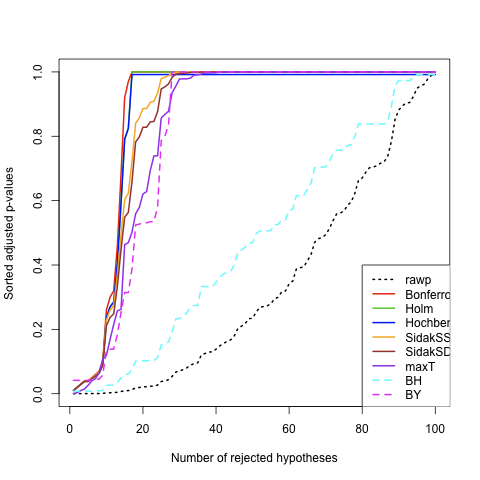
False Discovery Rate (FDR) is tightly linked to the preliminary example used when talking about the multtest package. In fact, when we plotted the adjusted p-values against the number of rejected hypotheses, we were already talking about the proportion of correct rejection of the null hypothesis. Here, “correct” means that the significant tests of hypothesis really reflects the reality, that is the true population parameters.
References
- Feise, R.J. (2002). Do multiple outcome measures require p-value adjustment? BMC Medical Research Methodology, 2: 8.
- Westfall, P.H., Tobias, R.D., Rom, D., Wolfinger, R.D., and Hochberg, Y. (1999). Multiple Comparisons and Multiple Tests Using the SAS System. Cary, NC: SAS Institute Inc., page 153.
- Westfall, P.H. (2005). Advances in Multiple Comparisons and Multiple Tests using the SAS System. Sugi, 25: Paper 264.
- Bretz, F., Genz, A. and Hothorn, L.A. (2001), On the numerical availability of multiple comparison procedures. Biometrical Journal, 43(5): 645–656.
- Hothorn, T., Bretz, F. and Westfall, P. (2008). Simultaneous Inference in General Parametric Models. Department of Statistics: Technical Reports, Nr. 19.
- Toothaker, L. (1993). Multiple Comparison Procedures. Sage University Paper, 89.
- Dudoit, S. and van der Laan, M.J. (2008). Multiple Testing Procedures with Applications to Genomics. Springer.
- Christensen, R. (2002). Plane Answers to Complex Questions, The Theory of Linear Models (3rd Ed.). Springer.
- Falissard, B. (2005). Comprendre et utiliser les statistiques dans les sciences de la vie (2nd Ed.). Masson.