High-dimensional data analysis in cancer research

August 9, 2010

This is a recent book co-edited by Xiaochun Li and Ronghui Xu (Springer, 2009) about feature selection and model validation in the context of oncological studies. More precisely, the seven chapters cover (snip).

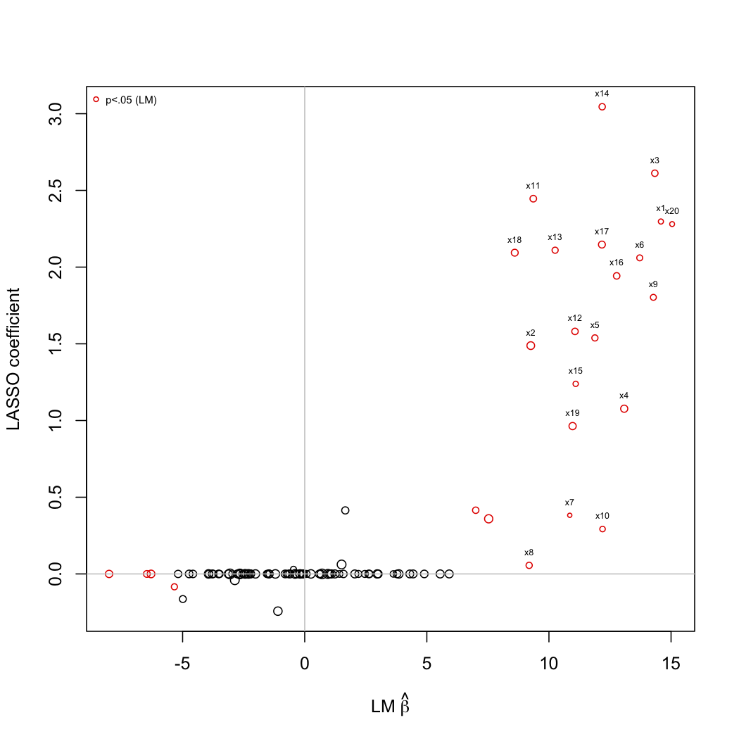
Here is a small simulation with LASSO penalization. The following picture depicts the coefficients estimated from simple univariate linear regression (x-axis) plotted against those estimated with LARS algorithm (LASSO mode). R code is shown below:

	# Time-stamp: <2010-08-10 11:51:15 chl>

	#
	# Illustration of LASSO penalization in multiple regression.
	#
	# The exemple is largely inspired from Harezlak, Tchetgen
	# and Li, Variable selection in regression -- Estimation,
	# Prediction, Sparsity, Inference,
	# in _High-Dimensional Data Analysis in Cancer Research_
	# (Ed. X. Li and R. Xu), Chapter 2, pp. 13--33.
	#

	library(MASS)
	library(lars)
	library(lasso2)

	n <- 50 # No. subjects
	p <- 100 # No. predictors
	s <- 20 # No. predictors in the active set
	rho <- 0.3 # introduce some colinearity among predictors
	mu <- rep(0,p) # all predictors are centred
	noise <- rnorm(n, 0, 2)
	# compound symmetry Sigma matrix (whole set of predictors)
	# Sigma <- rho*matrix(rep(1, p^2), p) + diag(rep(1-rho, p))

	# restrict colinearity to active set, e.g.
	#
	# s
	# +---+---+
	# \| Q \| 0 \|
	# +---+---+
	# p-s \| 0 \| P \|
	# +---+---+
	Q <- rho*matrix(rep(1,s^2),s)+diag(rep(1-rho,s))
	P <- 0*matrix(rep(1,(p-s)^2),p-s)+diag(rep(1,p-s))
	Sigma <- rbind(cbind(Q,matrix(0,nr=s,nc=p-s)),
	cbind(matrix(0,nr=p-s,nc=s),P))

	X <- mvrnorm(n, mu, Sigma)
	beta <- numeric(p)
	beta[1:s] <- runif(s, 0, 3)
	beta[(s+1):p] <- 0
	Y <- X%*%beta + noise

	# graphically check the structure of the <Y,X> block
	if (require(lattice)) {
	my.labs <- c("y",paste("x",seq(5,p+1,by=5),sep=""))
	levelplot(cor(cbind(Y,X)), xlab="", ylab="",
	scales=list(x=list(at=seq(1,p+1,by=5), labels=my.labs),
	y=list(at=seq(1,p+1,by=5), labels=my.labs)))
	}

	# mass univariate tests to screen interesting predictors
	beta.fit <- matrix(nr=p, nc=2, dimnames=list(NULL,c("est.","se")))
	for (i in 1:p)
	beta.fit[i,] <- summary(lm(Y~X[,i]-1))$coefficients[c(1,2)]

	# LARS solution
	xy.lars <- lars(X, Y, intercept=FALSE, use.Gram=FALSE)
	plot(xy.lars, breaks=FALSE)
	# use 10-fold CV to find optimal L1 parameter
	xy.lars.cv <- cv.lars(X, Y, trace=TRUE)
	xy.lars.frc <- lars.cv $fraction[xy.lars.cv$ cv.error==min(xy.lars.cv$cv.error)]
	xy.lars.coef <- coef(xy.lars, mode="fraction", s=lars.frc)

	# plot LM against LASSO estimates
	plot(beta.fit[,1], xy.lars.coef, cex=beta.fit[,2]/3,
	xlab=expression(paste("LM ",hat(beta))), ylab="LASSO coefficient",
	col=ifelse(abs(beta.fit[,1]/beta.fit[,2])>2, "red", "black"))
	text(beta.fit[1:s], xy.lars.coef[1:s], paste("x", 1:s, sep=""), cex=.5, pos=3)
	abline(v=0, h=0, col="gray")
	legend("topleft", c("p<.05 (LM)"), pch=1, col="red", bty="n", cex=.6)

view raw lasso.R hosted with ❤ by GitHub

Basically, I simulated a set of p=100 predictors, with s=20 variables (symmetrically correlated at 0.3) associated to the Y outcome. Then, I would like to see if LASSO penalization allows to recover the true associated Xs. Clearly, it seems to works quite well, except for some predictors which would be judged significant through univariate testing (although in this case, correcting for multiple comparisons with, e.g., Bonferroni, would yield an alpha of 5e-04).

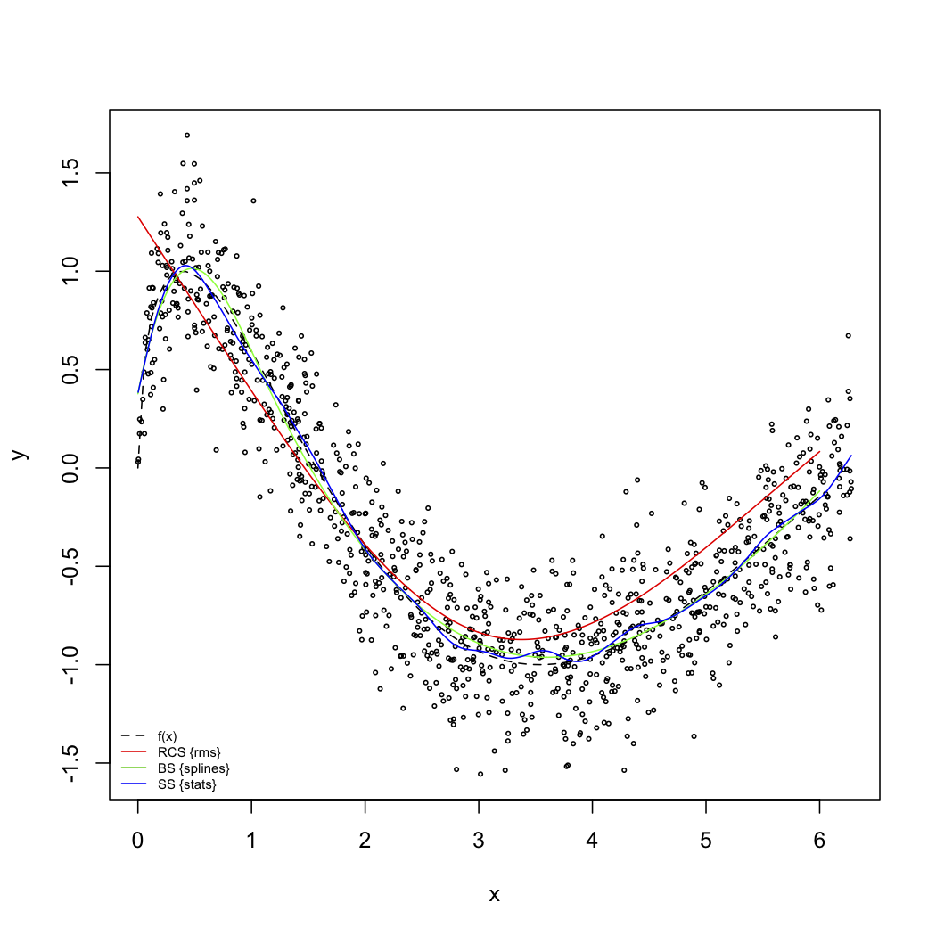
The next figure illustrates some nice properties of splines fitting. The code used to produce this picture follows.

	# Time-stamp: <2010-08-09 12:10:54 chl>

	#
	# Some illustrations of splines fitting.
	#
	# The example used throughout this script comes from
	# Kooperberg & LeBlanc, Multivariate Nonparametric Regression,
	# in _High-Dimensional Data Analysis in Cancer Research_
	# (Ed. X. Li and R. Xu), Chapter 3, p. 45.
	#

	library(rms)
	library(splines)
	set.seed(101)
	f <- function(x) sin(sqrt(2pix))
	n <- 1000
	x <- runif(n, 0, 2*pi)
	sigma <- rnorm(n, 0, 0.25)
	y <- f(x) + sigma
	plot(x, y, cex=.4)
	curve(f, 0, 6, lty=2, add=TRUE)
	# restricted cubic spline, 3 knots (2 Df)
	lm0 <- lm(y~rcs(x,3))
	lines(seq(0,6,length=1000),
	predict(lm0,data.frame(x=seq(0,6,length=1000))),
	col="red")
	# use B-spline and a single knot at x=1.13 (4 Df)
	lm1 <- lm(y~bs(x, knots=1.13))
	lines(seq(0,6,length=1000),
	predict(lm1,data.frame(x=seq(0,6,length=1000))),
	col="green")
	# cross-validated smoothed spline (approx. 20 Df)
	xy.spl <- smooth.spline(x, y, cv=TRUE)
	lines(xy.spl, col="blue")
	legend("bottomleft", c("f(x)","RCS {rms}","BS {splines}","SS {stats}"),
	col=1:4, lty=c(2,rep(1,3)),bty="n", cex=.6)

view raw splines.R hosted with ❤ by GitHub

aliquote.org

High-dimensional data analysis in cancer research

See Also