The Hmisc and rms packages
The Hmisc and rms packages provide a wide range of tools for data transformation, aggregated visual and numerical summaries, and enhanced R’s output for most common biostatistical models (linear regression, logistic or Cox regression).
Data preparation
Text-based data file (comma- or tab-delimited files) can be imported using
read.csv() or the more generic command read.table(). The foreign
package can be used to process binary data files from other statistical
packages. See also R Data Import/Export. Hmisc offers extended
support for foreign data files, including CSV (csv.get()), SAS
(sas.get()), SPSS (spss.get()), or Stata (stata.get()). Variables
names are automatically converted to lowercase, dates are generally better
handled. Documentation and additional information on the
Hmisc website. Various dataset can be download from a
public repository via the getHdata() command.
As always, before using any package in R, it must be loaded first:
library(Hmisc)
## help(package = Hmisc)
In what follows, we will be using birthwt data set from the MASS
package. The low birth weight study is one of the datasets used throughout
Hosmer and Lemeshow’s textbook on Applied Logistic Regression (2000, Wiley,
2nd ed.). The goal of this prospective study was to identify risk factors
associated with giving birth to a low birth weight baby (weighing less than
2,500 grams). Data were collected on 189 women, 59 of which had low birth
weight babies and 130 of which had normal birth weight babies. Four
variables which were thought to be of importance were age, weight of the
subject at her last menstrual period, race, and the number of physician
visits during the first trimester of pregnancy. It can be loaded as shown
below:
data(birthwt, package = "MASS")
## help(birthwt)
In this data set there is no missing observations, but let introduce
some NA values. Note that variable names are relatively short and poorly
informative. Shorter names are, however, easy to manipulate with R. Hmisc
provides specific command for labeling (label()) and adding units of
measurement (units()) as additional attributes to a given variable (or
data frame). We will also convert some of the variables as factor with
proper label (rather than 0/1 values) to facilitate reading of summary
tables or subsequent graphics.
birthwt$age[5] <- NA
birthwt$ftv[sample(1:nrow(birthwt), 5)] <- NA
yesno <- c("No", "Yes")
birthwt <- within(birthwt, {
    smoke <- factor(smoke, labels = yesno)
    low <- factor(low, labels = yesno)
    ht <- factor(ht, labels = yesno)
    ui <- factor(ui, labels = yesno)
    race <- factor(race, levels = 1:3, labels = c("White", "Black", "Other"))
    lwt <- lwt/2.2  ## weight in kg
})
label(birthwt$age) <- "Mother age"
units(birthwt$age) <- "years"
label(birthwt$bwt) <- "Baby weight"
units(birthwt$bwt) <- "grams"
label(birthwt, self = TRUE) <- "Hosmer & Lemeshow's low birth weight study."
list.tree(birthwt)  ## equivalent to str(birthwt)
##  birthwt = list 10 (24584 bytes)( data.frame )
## .  low = integer 189= category (2 levels)( factor )= No No No No No No ...
## .  age = integer 189( labelled )= 19 33 20 21 NA 21 ...
## . A  label = character 1= Mother age
## . A  units = character 1= years
## .  lwt = double 189= 82.727 70.455 47.727 ...
## .  race = integer 189= category (3 levels)( factor )= Black Other White ...
## .  smoke = integer 189= category (2 levels)( factor )= No No Yes Yes Yes ...
## .  ptl = integer 189= 0 0 0 0 0 0 0 0 ...
## .  ht = integer 189= category (2 levels)( factor )= No No No No No No ...
## .  ui = integer 189= category (2 levels)( factor )= Yes No No Yes Yes ...
## .  ftv = integer 189= 0 3 1 2 0 0 1 1 ...
## .  bwt = integer 189( labelled )= 2523 2551 2557 2594 ...
## . A  label = character 1= Baby weight
## . A  units = character 1= grams
## A  row.names = character 189= 85 86 87 88 89 91 92  ...
## A  label = character 1= Hosmer & Lemeshow's lo
The last command, list.tree(), offers a convenient replacement for R’s
str(), and in addition to variable type and a list of the first
observation for each variable it will display Hmisc labels associated to
them.
The contents() command offers a quick summary of data format and missing
values, and it provides a list of labels associated to variables treated as
factor by R.
contents(birthwt)
##
## Data frame:birthwt	189 observations and 10 variables    Maximum # NAs:5
##
##            Labels Units Levels Storage NAs
## low                          2 integer   0
## age    Mother age years        integer   1
## lwt                             double   0
## race                         3 integer   0
## smoke                        2 integer   0
## ptl                            integer   0
## ht                           2 integer   0
## ui                           2 integer   0
## ftv                            integer   5
## bwt   Baby weight grams        integer   0
##
## +--------+-----------------+
## |Variable|Levels           |
## +--------+-----------------+
## |  low   |No,Yes           |
## |  smoke |                 |
## |  ht    |                 |
## |  ui    |                 |
## +--------+-----------------+
## |  race  |White,Black,Other|
## +--------+-----------------+
Another useful command is describe(), which gives detailed summary
statistics for each variable in a given data frame. It can be printed as
HTML, or as PDF (by using the latex() backend), and in the latter case
small graphics are added that depict distribution of continuous variables.
describe(birthwt, digits = 3)
## birthwt
##
##  10  Variables      189  Observations
## ---------------------------------------------------------------------------
## low
##       n missing  unique
##     189       0       2
##
## No (130, 69%), Yes (59, 31%)
## ---------------------------------------------------------------------------
## age : Mother age [years]
##       n missing  unique    Mean     .05     .10     .25     .50     .75
##     188       1      24    23.3      16      17      19      23      26
##     .90     .95
##      31      32
##
## lowest : 14 15 16 17 18, highest: 33 34 35 36 45
## ---------------------------------------------------------------------------
## lwt
##       n missing  unique    Mean     .05     .10     .25     .50     .75
##     189       0      75      59    42.9    45.3    50.0    55.0    63.6
##     .90     .95
##    77.3    85.5
##
## lowest :  36.4  38.6  40.5  40.9  41.4
## highest:  97.7 104.1 106.8 109.5 113.6
## ---------------------------------------------------------------------------
## race
##       n missing  unique
##     189       0       3
##
## White (96, 51%), Black (26, 14%), Other (67, 35%)
## ---------------------------------------------------------------------------
## smoke
##       n missing  unique
##     189       0       2
##
## No (115, 61%), Yes (74, 39%)
## ---------------------------------------------------------------------------
## ptl
##       n missing  unique    Mean
##     189       0       4   0.196
##
## 0 (159, 84%), 1 (24, 13%), 2 (5, 3%), 3 (1, 1%)
## ---------------------------------------------------------------------------
## ht
##       n missing  unique
##     189       0       2
##
## No (177, 94%), Yes (12, 6%)
## ---------------------------------------------------------------------------
## ui
##       n missing  unique
##     189       0       2
##
## No (161, 85%), Yes (28, 15%)
## ---------------------------------------------------------------------------
## ftv
##       n missing  unique    Mean
##     184       5       6   0.799
##
##            0  1  2 3 4 6
## Frequency 97 46 29 7 4 1
## %         53 25 16 4 2 1
## ---------------------------------------------------------------------------
## bwt : Baby weight [grams]
##       n missing  unique    Mean     .05     .10     .25     .50     .75
##     189       0     131    2945    1801    2038    2414    2977    3487
##     .90     .95
##    3865    3997
##
## lowest :  709 1021 1135 1330 1474, highest: 4167 4174 4238 4593 4990
## ---------------------------------------------------------------------------
Of course, it is also possible to describe only a subset of the data or specific data.
describe(subset(birthwt, select = c(age, race, bwt, low)))
Hmisc has several helper functions to work with categorical variables,
like dropUnusedLevels() to remove missing levels or Cs() to convert
unquoted list of variables names to characters. It also provides a
replacement for R’s cut() function with better default options (especially
the infamous include.lowest=FALSE) to discretize a continuous
variable. Here are some examples of use:
table(cut2(birthwt$lwt, g = 4))
##
## [36.4, 50.9) [50.9, 55.5) [55.5, 64.1) [64.1,113.6]
##           53           43           46           47
table(cut2(birthwt$age, g = 3, levels.mean = TRUE))
##
## 18.074 23.091 30.019
##     68     66     54
Using levels.mean=TRUE will return class center, instead of class
intervals.
There are also a bunch of command dedicated to variables clustering,
analysis of missing patterns, or simple (impute()) or multiple
(aregImpute(), transcan()) imputation methods. Here is how we would
impute missing values with the median in the case of a continuous variable:
lwt <- birthwt$lwt
lwt[sample(length(lwt), 10)] <- NA
lwt.i <- impute(lwt)
summary(lwt.i)
##
##  10 values imputed to 55
##    Min. 1st Qu.  Median    Mean 3rd Qu.    Max.
##    36.4    50.0    55.0    59.0    63.6   114.0
Missing observations will be marked with an asterisk when we print the whole
object in R. To use the mean instead of the median, we just have to add the
fun=mean option.
Visual and numerical summaries
There are three useful commands that provide summary statistics for a list of variables. They implement the split-apply-combine strategy in the spirit of R’s built-in functions (unlike plyr).
The first one, summarize(), can be seen as an equivalent to R’s
aggregate() command. Given a response variable and one or more
classification factors, it applies a specific function to all data chunk,
where each chunk is defined based on factor levels. The results are stored
in a matrix, which can easily be coerced to a data frame (as.data.frame()
or Hmisc::matrix2dataFrame()).
Remark: Some of the results are shown via the prn() command.
f <- function(x, na.opts = TRUE) c(mean = mean(x, na.rm = na.opts), sd = sd(x,
    na.rm = na.opts))
out <- with(birthwt, summarize(bwt, race, f))
##
## Average baby weight by ethnicity   out
##
##    race  bwt    sd
## 3 White 3103 727.9
## 1 Black 2720 638.7
## 2 Other 2805 722.2
Contrary to aggregate(), this command provides multiway data structure in
case we ask to compute more than one quantity, as the following command will
confirm:
dim(out) ## should have 3 columns
## [1] 3 3
dim(aggregate(bwt ~ race, data = birthwt, f))
## [1] 3 2
Summarizing multivariate responses or predictors is also possible, with
either summarize() or mApply(). Of course, any built-in functions, such
as colMeans() could be used in place of our custom summary command.
with(birthwt, summarize(bwt, llist(race, smoke), f))
##    race smoke  bwt    sd
## 5 White    No 3429 710.1
## 6 White   Yes 2827 626.5
## 1 Black    No 2854 621.3
## 2 Black   Yes 2504 637.1
## 3 Other    No 2816 709.3
## 4 Other   Yes 2757 810.0
The second command, bystats(), (or bystats2() for two-way tabular
output) allows to describe with any custom or built-in function one or
multiple outcome by two explanatory variables, or even more. Sample size and
the number of missing values are also printed.
with(birthwt, bystats(cbind(bwt, lwt), smoke, race))
##
##  Mean of cbind(bwt, lwt) by smoke
##
##             N  bwt   lwt
## No White   44 3429 63.11
## Yes White  52 2827 57.41
## No Black   16 2854 67.93
## Yes Black  10 2504 64.82
## No Other   55 2816 54.16
## Yes Other  12 2757 56.36
## ALL       189 2945 59.01
with(birthwt, bystats2(lwt, smoke, race))
##
##  Mean of lwt by smoke
##
## +----+
## |N   |
## |Mean|
## +----+
## +---+-----+-----+-----+-----+
## |No | 44  | 16  | 55  |115  |
## |   |63.11|67.93|54.16|59.50|
## +---+-----+-----+-----+-----+
## |Yes| 52  | 10  | 12  | 74  |
## |   |57.41|64.82|56.36|58.24|
## +---+-----+-----+-----+-----+
## |ALL| 96  | 26  | 67  |189  |
## |   |60.02|66.73|54.55|59.01|
## +---+-----+-----+-----+-----+
The third and last command is summary.formula(), which can be abbreviated
as summary() as long as formula is used to describe variables
relationships. There are three main configurations (method=):
"response", where a numerical variable is summarized for each level of
one or more variables (numerical variables will be discretized in 4
classes), as summarize() does; "cross", to compute conditional and
marginal means of several response variables described by at most 3
explanatory variables (again, continuous predictors are represented as
quartiles); "reverse", to summarize univariate distribution of a set of
variables for each level of a classification variable (which appears on the
left-hand side of the formula). Variables are viewed as continuous as long
as they have more than 10 distinct values, but this can be changed by
setting, e.g., continuous=5. With method="reverse", it is possible to
add overall=TRUE, test=TRUE to add overall statistics and corresponding
statistical tests of null effect between the groups.
Here are some examples of use.
summary(bwt ~ race + ht + lwt, data = birthwt)
## Baby weight    N=189
##
## +-------+------------+---+----+
## |       |            |N  |bwt |
## +-------+------------+---+----+
## |race   |White       | 96|3103|
## |       |Black       | 26|2720|
## |       |Other       | 67|2805|
## +-------+------------+---+----+
## |ht     |No          |177|2972|
## |       |Yes         | 12|2537|
## +-------+------------+---+----+
## |lwt    |[36.4, 50.9)| 53|2656|
## |       |[50.9, 55.5)| 43|3059|
## |       |[55.5, 64.1)| 46|3075|
## |       |[64.1,113.6]| 47|3038|
## +-------+------------+---+----+
## |Overall|            |189|2945|
## +-------+------------+---+----+
summary(cbind(lwt, age) ~ race + bwt, data = birthwt, method = "cross")
##
##  mean by race, bwt
##
## +-------+
## |N      |
## |Missing|
## |lwt    |
## |age    |
## +-------+
## +-----+-----------+-----------+-----------+-----------+-----+
## | race|[ 709,2424)|[2424,3005)|[3005,3544)|[3544,4990]| ALL |
## +-----+-----------+-----------+-----------+-----------+-----+
## |White|    19     |    23     |    20     |    33     | 95  |
## |     |   0       |   1       |   0       |   0       |1    |
## |     |   55.55   |   57.67   |   62.23   |   63.25   |60.14|
## |     |   22.74   |   24.78   |   24.50   |   24.91   |24.36|
## +-----+-----------+-----------+-----------+-----------+-----+
## |Black|     9     |     9     |     6     |     2     | 26  |
## |     |   0       |   0       |   0       |   0       |0    |
## |     |   65.10   |   59.70   |   70.83   |   93.41   |66.73|
## |     |   23.44   |   20.89   |   20.00   |   20.50   |21.54|
## +-----+-----------+-----------+-----------+-----------+-----+
## |Other|    20     |    16     |    19     |    12     | 67  |
## |     |   0       |   0       |   0       |   0       |0    |
## |     |   51.23   |   52.95   |   58.90   |   55.34   |54.55|
## |     |   22.20   |   22.69   |   22.26   |   22.50   |22.39|
## +-----+-----------+-----------+-----------+-----------+-----+
## |ALL  |    48     |    48     |    45     |    47     |188  |
## |     |   0       |   1       |   0       |   0       |1    |
## |     |   55.54   |   56.48   |   61.97   |   62.51   |59.06|
## |     |   22.65   |   23.35   |   22.96   |   24.11   |23.27|
## +-----+-----------+-----------+-----------+-----------+-----+
summary(low ~ race + ht, data = birthwt, fun = table)
## low    N=189
##
## +-------+-----+---+---+---+
## |       |     |N  |No |Yes|
## +-------+-----+---+---+---+
## |race   |White| 96| 73|23 |
## |       |Black| 26| 15|11 |
## |       |Other| 67| 42|25 |
## +-------+-----+---+---+---+
## |ht     |No   |177|125|52 |
## |       |Yes  | 12|  5| 7 |
## +-------+-----+---+---+---+
## |Overall|     |189|130|59 |
## +-------+-----+---+---+---+
out <- summary(low ~ race + age + ui, data = birthwt, method = "reverse", overall = TRUE,
    test = TRUE)
print(out, prmsd = TRUE, digits = 2)
##
##
## Descriptive Statistics by low
##
## +------------------+---+----------------------------+----------------------------+----------------------------+----------------------------+
## |                  |N  |No                          |Yes                         |Combined                    |  Test                      |
## |                  |   |(N=130)                     |(N=59)                      |(N=189)                     |Statistic                   |
## +------------------+---+----------------------------+----------------------------+----------------------------+----------------------------+
## |race : White      |189|          56% (73)          |          39% (23)          |          51% (96)          | Chi-square=5 d.f.=2 P=0.082|
## +------------------+---+----------------------------+----------------------------+----------------------------+----------------------------+
## |    Black         |   |          12% (15)          |          19% (11)          |          14% (26)          |                            |
## +------------------+---+----------------------------+----------------------------+----------------------------+----------------------------+
## |    Other         |   |          32% (42)          |          42% (25)          |          35% (67)          |                            |
## +------------------+---+----------------------------+----------------------------+----------------------------+----------------------------+
## |Mother age [years]|188| 19.0/23.0/28.0  23.7+/- 5.6| 19.5/22.0/25.0  22.3+/- 4.5| 19.0/23.0/26.0  23.3+/- 5.3|   F=1.5 d.f.=1,186 P=0.22  |
## +------------------+---+----------------------------+----------------------------+----------------------------+----------------------------+
## |ui : Yes          |189|          11% ( 14)         |          24% ( 14)         |          15% ( 28)         |Chi-square=5.4 d.f.=1 P=0.02|
## +------------------+---+----------------------------+----------------------------+----------------------------+----------------------------+
Note also that tabular output can be converted to graphical displays by
using plot() like in, e.g.,
plot(out, which = "categorical")
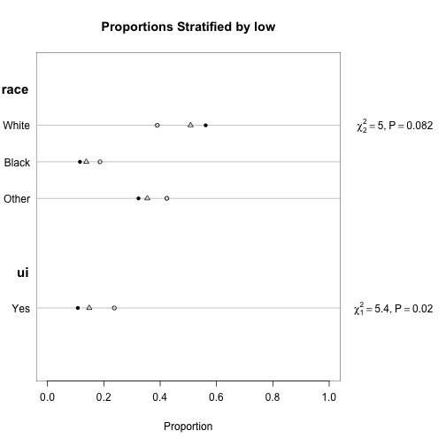
Hmisc provides replacement for some lattice commands, in particular
xYplot() and dotchart2(), or Dotplot(). In fact, it is also its
strength because we do not need to learn ggplot2 to overcome base
graphics limitations, and using Hmisc keep in line with lattice charts
(and their multiple options).
Let say we would like to display average birth weight plus or minus one standard error for each class of mother ethnicity. Assuming there is no missing variable we could define a simple function that returns means and associated lower/upper bounds.
se <- function(x) sd(x)/sqrt(length(x))
f <- function(x) c(mean = mean(x), lwr = mean(x) - se(x), upr = mean(x) + se(x))
d <- with(birthwt, summarize(bwt, race, f))
##
## Summary statistics (Mean +/- SE) by group   d
##
##    race  bwt  lwr  upr
## 3 White 3103 3028 3177
## 1 Black 2720 2594 2845
## 2 Other 2805 2717 2894
xYplot(Cbind(bwt, lwr, upr) ~ numericScale(race, label = "Ethnicity"), data = d,
    type = "b", keys = "lines", ylim = range(apply(d[, 3:4], 2, range)) + c(-1,
        1) * 100, scales = list(x = list(at = 1:3, labels = levels(d$race))))
An easier (also shorter) solution is to rely on lattice extra commands, like
library(latticeExtra)
segplot(race ~ lwr + upr, data = d, centers = bwt, horizontal = FALSE, draw.bands = FALSE,
    ylab = "Baby weight (g)")
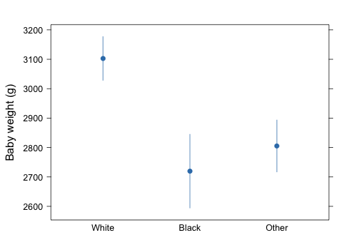
although xYplot() is very handy when processing model predictions
generated by ols() or lrm(), as we will discuss below.
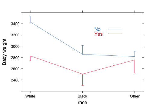
Hmisc provides automatic labelling of curves or levels of grouping factor,
which are used as in standard lattice graphics (groups=), without the need
to rely on the directlabels package.
d <- with(birthwt, summarize(bwt, llist(race, smoke), f))
xYplot(Cbind(bwt, lwr, upr) ~ numericScale(race), groups = smoke, data = d,
    type = "l", keys = "lines", method = "alt bars", ylim = c(2200, 3600), scales = list(x = list(at = 1:3,
        labels = levels(d$race))))
Model fitting and diagnostic
The rms package is used in combination with Hmisc, which takes care
of data pre-processing and statistical summary. It is devoted to model
fitting, including validation (validate()) and calibration (calibrate())
using bootstrap. It further includes utilities to refine general modeling
strategies and to handle higher-order terms (polymonial or restricted cubic
splines) or ordered catgeorical predictors, see online
help(rms.trans). The definitive guide to regression modeling using rms is
Harrell, F.E., Jr (2001). Regression Modeling Strategies, With Applications to Linear Models, Logistic Regression, and Survival Analysis. Springer.
The companion website is BIOS 330: Regression Modeling Strategies.
Instead of lm(), we will use ols() to perform linear regression, but the
general formulation of the parametric model remains the same: a formula is
used to describe variable relationships (the response variable is on the
left-hand side, while predictors are on the right-hand side). A basic usage
of this command is shown below. To reuse the model for predictions purpose,
the linear predictor must be stored with model results (x=TRUE).
library(rms)
m <- ols(bwt ~ age + race + ftv, data = birthwt, x = TRUE)
m
##
## Linear Regression Model
##
## ols(formula = bwt ~ age + race + ftv, data = birthwt, x = TRUE)
##
## Frequencies of Missing Values Due to Each Variable
##  bwt  age race  ftv
##    0    1    0    5
##
##
##                   Model Likelihood     Discrimination
##                      Ratio Test           Indexes
## Obs        183    LR chi2     10.37    R2       0.055
## sigma 725.0771    d.f.            4    R2 adj   0.034
## d.f.       178    Pr(> chi2) 0.0347    g      192.508
##
## Residuals
##
## Baby weight [grams]
##        Min         1Q     Median         3Q        Max
## -2132.2374  -499.8035     0.9503   520.4314  1759.2352
##
##            Coef      S.E.     t     Pr(>|t|)
## Intercept  2957.5528 261.1681 11.32 <0.0001
## age           5.7498  10.5102  0.55 0.5850
## race=Black -373.3901 163.1956 -2.29 0.0233
## race=Other -295.6800 120.0166 -2.46 0.0147
## ftv          14.4698  51.8045  0.28 0.7803
Note that, contrary to lm(), the summary() method (or more precisely,
summary.rms()) does something else. With ols() it will print a summary
of the effect of each factor. It requires, however, that the user create a
datadist object to store values for the predictors entering the
model, and that object must be available in the current namespace. So, the
preceding example becomes:
d <- datadist(birthwt)
options(datadist = "d")
m <- ols(bwt ~ age + race + ftv, data = birthwt, x = TRUE)
summary(m)
##              Effects              Response : bwt
##
##  Factor             Low High Diff. Effect  S.E.   Lower 0.95 Upper 0.95
##  age                19  26    7      40.25  73.57 -103.95    184.45
##  ftv                 0   1    1      14.47  51.80  -87.07    116.00
##  race - Black:White  1   2   NA    -373.39 163.20 -693.25    -53.53
##  race - Other:White  1   3   NA    -295.68 120.02 -530.91    -60.45
Effect size measures can also be displayed graphically using the
corresponding plot method:
plot(summary(m))
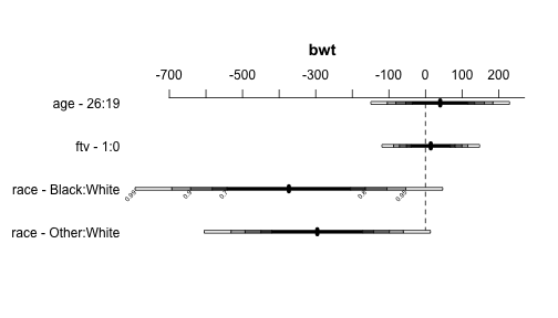
Note also that in the case of multiple regression it is possible to select baseline category and adjust the effect for a particular value of a continuous predictor, as in the example below.
summary(m, race = "Other", age = median(birthwt$age))
##              Effects              Response : bwt
##
##  Factor             Low High Diff. Effect S.E.   Lower 0.95 Upper 0.95
##  age                19  26    7     40.25  73.57 -103.95    184.4
##  ftv                 0   1    1     14.47  51.80  -87.07    116.0
##  race - White:Other  3   1   NA    295.68 120.02   60.45    530.9
##  race - Black:Other  3   2   NA    -77.71 169.55 -410.02    254.6
A more conventional ANOVA table for the regression can be obtained using
anova().
anova(m)
##                 Analysis of Variance          Response: bwt
##
##  Factor     d.f. Partial SS MS      F    P
##  age          1    157346    157346 0.30 0.5850
##  race         2   4529519   2264760 4.31 0.0149
##  ftv          1     41017     41017 0.08 0.7803
##  REGRESSION   4   5454889   1363722 2.59 0.0381
##  ERROR      178  93581138    525737
Measures of influence are available with the which.influence() command,
and it returns observations that are above a certain threshold with respect
to their DFBETA (default, 0.2). The vif() command displays variance
inflation factor, which can be used to gauge multicolinearity issue.
which.influence(m)
## $Intercept
## [1] 117 130 131 133
##
## $age
## [1] 110 127 130 131 133 141
##
## $race
## [1] 106 110 131 133 134 138
##
## $ftv
## [1]  68 110 133
vif(m)
##        age race=Black race=Other        ftv
##      1.092      1.130      1.132      1.056
Model predictions are carried out the R’s way, using fitted(), or
rms::Predict. The latter offers additional control over adjustment factor
(like the effects package does), and does not require to create a data
frame as in predict(). It also handles 95% confidence intervals smoothly.
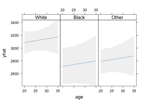
p <- Predict(m, age = seq(20, 35, by = 5), race, ftv = 1)
xYplot(Cbind(yhat, lower, upper) ~ age | race, data = p, layout = c(3, 1), method = "filled bands",
    type = "l", col.fill = gray(0.95))
lrm() function, and it works almost
in the same way, except that it provides more convenient output than R’s
glm(), especially in terms of adjusted odds-ratio, partial effects,
confidence intervals, or likelihhod ratio test.
A very comprehensive introduction to Frank Harrell’s packages has been published recently: An Introduction to the Harrell“verse”: Predictive Modeling using the Hmisc and rms Packages.