Lasso Regression with Stata
Here comes the time of lasso and elastic net regression with Stata.
While ridge estimators have been available for quite a long time now (ridgereg), the class of estimators developped by Friedman, Hastie and Tibshirani has long been missing in Stata. It looks like it is now available in the elasticregress package (also available on GitHub), at least for linear models.
Here is a toy example, inspired from a previous talk (PDF) I gave on the topic. Basically, the ridge or L2 penalty consists in shrinking parameter estimates toward zero in order to stabilize their variance. The amount of shrinkage is controlled by the penalty parameter, $\lambda$, such that it is possible to make the estimates tend towards 0 by using a very high lambda value as demonstrated below using a polynomial model of order $k$: The yellow points are the observed values and the blue ones are predictions from this model with varying amount of shrinkage.
The Lasso penalty on the contrary will simply set the parameter estimates to zero past a certain threshold, which makes it convenient when one thinks in terms of variable selection although this technique does not lend itself well to collinearity, in which case the elasticnet criterion is certainly a better option.
Let us assume we have a sample of $n$ observations generated from the following model:
$$ y = \beta_0 + \sum_{j=1}^{10}\beta_jx_j + u, $$
where $u$ are random gaussian perturbations and $n=50$.
clear
set seed 101
set obs 50
forvalues j = 1/10 {
  generate x`j' = rnormal(0,1)
}
generate y = 1.1*x1 + 0.8*x2 - 0.7*x5 + 1.4*x6 + rnormal(0,1)
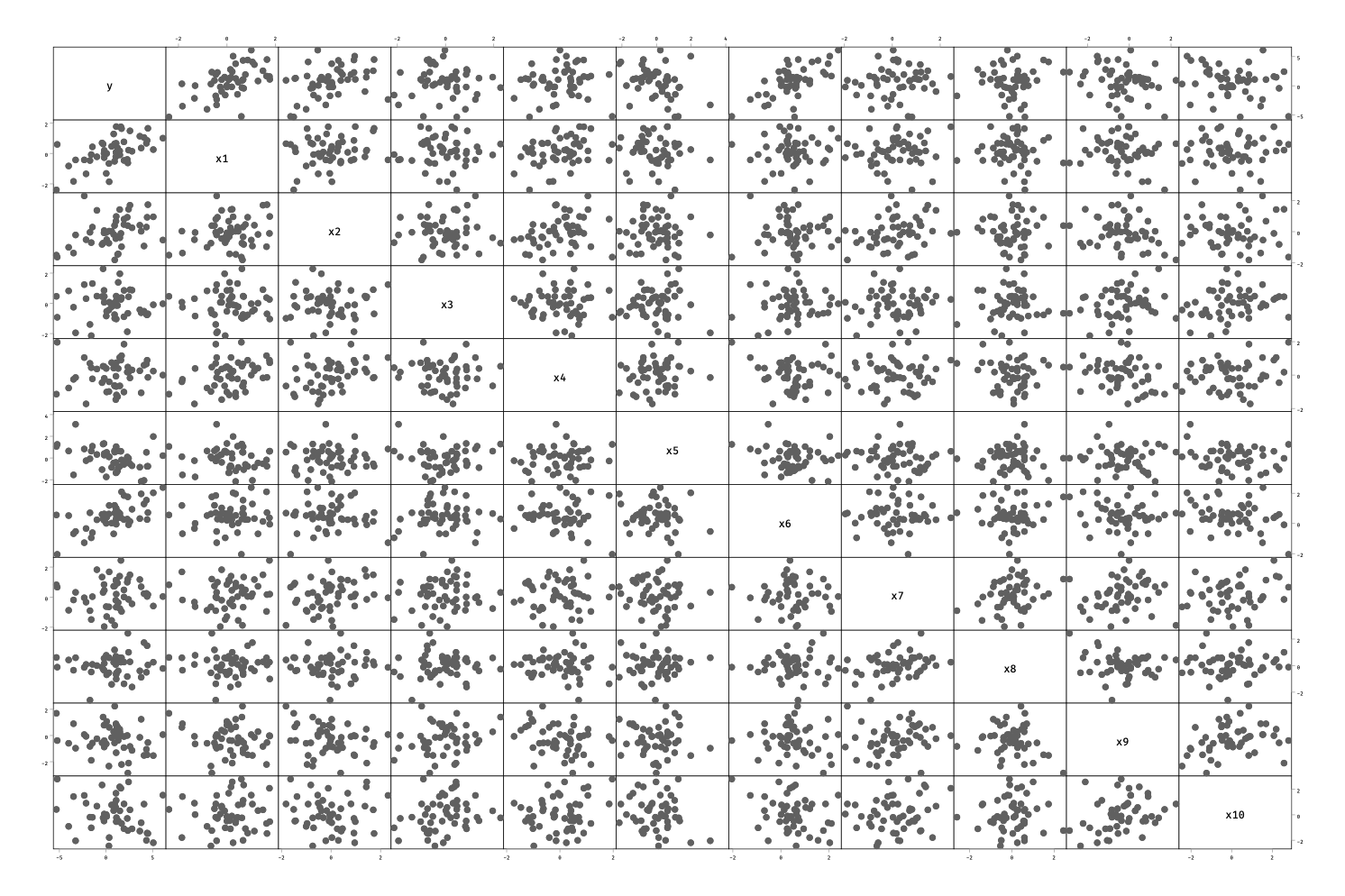
graph matrix y x*
Note that in the above model, we do not control the variance-covariance matrix of the predictors so that we can’t ensure that the partial correlations are exactly zero. More appropriate techniques are available to create multivariate normal observations. It is easy to check visually that the correlation matrix between the outcome $y$ and the predictors $x_j$ behave as expected:

And here is what we get when using a combination of L1 and L2 penalties:
. elasticregress y x*
Warning: the smallest λ tested was the MSE-minimising λ.
Consider re-running estimation with a smaller epsilon.

Elastic-net regression                 Number of observations     =         50
                                       R-squared                  =     0.8138
                                       alpha                      =     1.0000
                                       lambda                     =     0.0918
                                       Cross-validation MSE       =     1.6373
                                       Number of folds            =         10
                                       Number of alpha tested     =          6
                                       Number of lambda tested    =        100
------------------------------------------------------------------------------
           y |      Coef.
-------------|----------------------------------------------------------------
          x1 |   1.131193
          x2 |   .6925592
          x3 |  -.0984186
          x4 |          0
          x5 |  -.5039949
          x6 |   1.490665
          x7 |          0
          x8 |   .1432863
          x9 |          0
         x10 |  -.1665392
       _cons |  -.1164585
------------------------------------------------------------------------------
. display e(lambda)
.09181307
The estimates are stored in the e(b) vector, and more options are available. Here is one way to improve our original estimates, by increasing the grid search size from cross-validation and considering the $\pm 1$ SE rule:
. elasticregress y x*, numalpha(10) epsilon(0.00001) lambda1se

Elastic-net regression                 Number of observations     =         50
                                       R-squared                  =     0.7853
                                       alpha                      =     0.6667
                                       lambda                     =     0.2351
                                       Cross-validation MSE       =     1.9336
                                       Number of folds            =         10
                                       Number of alpha tested     =         10
                                       Number of lambda tested    =        100
------------------------------------------------------------------------------
           y |      Coef.
-------------|----------------------------------------------------------------
          x1 |   1.012981
          x2 |   .5975951
          x3 |          0
          x4 |          0
          x5 |  -.4317686
          x6 |    1.34201
          x7 |          0
          x8 |   .0574305
          x9 |          0
         x10 |  -.1385899
       _cons |  -.0239716
------------------------------------------------------------------------------