As I was re-reading an old book of mathematical statistics by van der Waerden,¹ I found this little gem in the chapter dealing with the method of ordinary least squares. It is interesting because even if the purpose of this textbook is to expose the basis of mathematical statistics, most of the examples remain anchored in real-life or historical example. I rarely encountered such a pragmatic approach combining theoretical development and applied reasoning in more recent textbooks.

Here’s a quick translation from French to English (bear in mind that I’m not a native speaker nor an expert in astronomy).

Here is a screenshot of the data table:

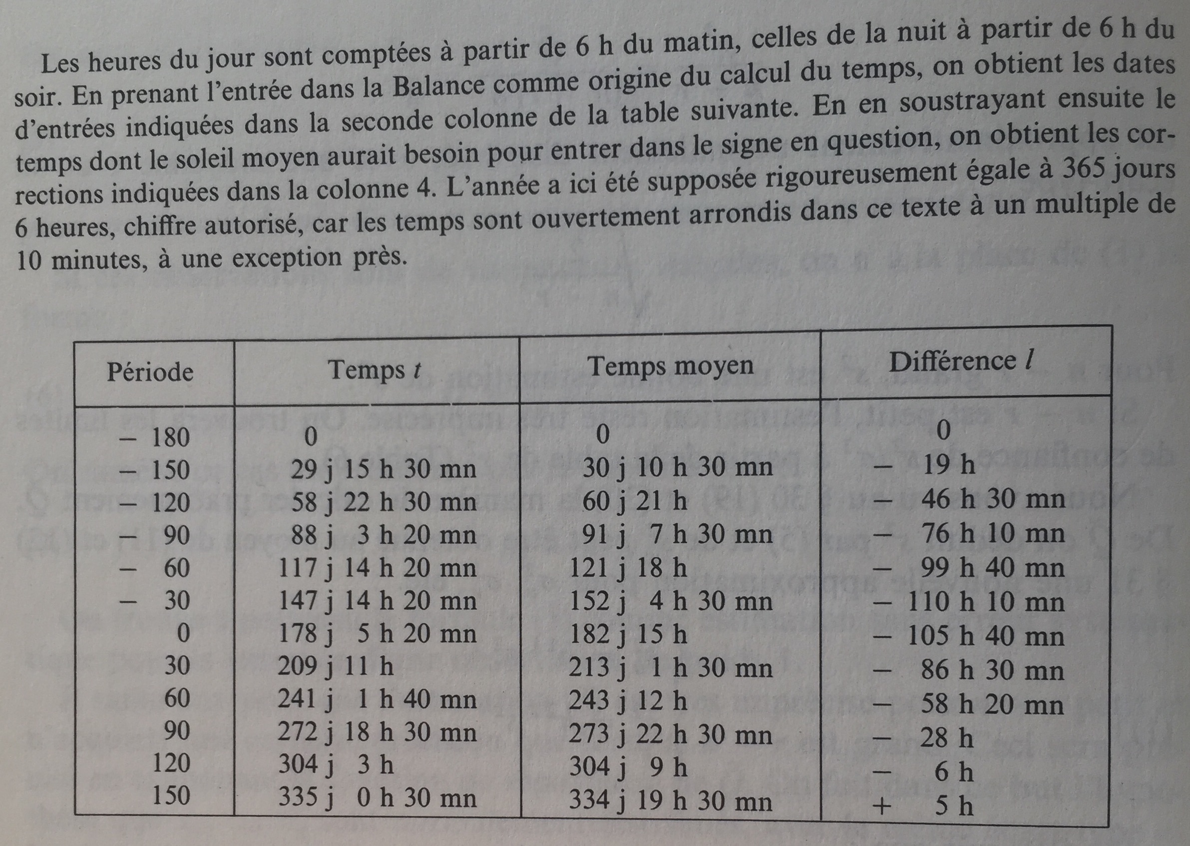
These values were derived from a Byzantine calendar where the dates entered in the twelve signs of the zodiac were recorded in the form of hours, the hours of the day being counted from 6 a.m. onwards and the sign of Libra being considered as the origin of the calculation of time. We then subtracted the time that the average sun would need to enter the sign in question, assuming a year strictly equal to 365 days and 6 hours.

Let us denote $\lambda$ the width of the sun at the entrance to a zodiac sign, and $\alpha$ the length of the apogee. The difference $\chi = \lambda - \alpha$ is called the true anomaly. The length of the arc of the apogee $A$ of eccentricity to the sun $S$ is called the mean anomaly. It will be denoted by $x + \omega$. The difference $\omega$ between the true anomaly and the mean anomaly is called the mean point equation. If $e$ is the eccentricity, the following equality between $\omega$ and $x$ follows from the sinus rule:

$$\sin \omega = e \sin x$$

or $\omega = \text{arc}\hskip-.15ex\sin (e \sin x)\hskip.15ex$, as illustrated in the picture below.

Since $e$ is small, $\text{arc}\hskip-.15ex\sin$ can be expanded as a power series up to the 2nd term:

$$\begin{align*} \omega &= e \sin x + \frac{1}{6}e^3 \sin^3 x \cr &= e \sin x + \frac{1}{24}e^3 (3 \sin x - \sin 3x) \cr &= \left(e + \frac{1}{8}e^3\right) \sin x - \frac{1}{24}e^3 \sin 3x \end{align*}$$

The time needed by the sun to travel the arc $x + \omega$ on the eccentricity is $t = \frac{T}{2\pi}(x + \omega)$, where $T = 365.25$ days is the total traveling time. For an average movement, the time would be $t_0 = \frac{T}{2\pi}x$. The differences $t-t_0 = \frac{T}{2\pi}\omega$ must be equal to the values $l$ in the last column of the table in the above screenshot, upon addition of an unknown constant $d$ and a corrective term, unknown, resulting from calculus and rounding errors. We have:

$$\frac{T}{2\pi} \omega + d = l + k.$$

Substituting the preceding expression for $\omega$, we get:

$$a \sin x + b \sin 3x + d = l + k$$

with

$$\left\{\begin{align*} a &= \frac{T}{2\pi} \left( e + \frac{1}{8}e^3\right)\cr b &= - \frac{T}{2\pi} \frac{1}{24}e^3 = - ce^3 \end{align*}\right.$$

where $c$ is known. Let us denote $x = \lambda - \alpha$, we finally have the following equation:

$$a \sin (\lambda - \alpha) + b \sin 3 (\lambda - \alpha) + d = l + k.$$

Since the 12 lengths $\lambda$ and the values $l$ from the table are known, we have 12 “equations of observations” with three unknowns, $e$, $\alpha$ and $d$. They will be determined so that $k_1^2 + \dots + k_{12}^2$ be as small as possible.

First, we can neglect the term $b$. One we get an approximatio for $e$, we obtain $b = -ce^3$, and the term $b$ can be moved in the RHS in order to perform a second approximation for $a$, which happens to be identical to the first one since the terms involving $\sin 3x$ vanish in the normal equations. The term in $b$ can thus be discarded and we will write:

$$a \sin \lambda \cos \alpha - a \cos \lambda \sin \alpha + d = l + k.$$

After we introduce the new unknowns :

$$\left\{\begin{align*} u &= a \cos \alpha \cr v &= -a \sin \alpha \cr w &= d \end{align*}\right.$$

we get 12 linear equations of the form $u \sin \lambda + v \cos \lambda + w = l + k$, and the normal equations can be written as follows:

$$\left\{\begin{array}{l} [aa]u + [ab]v + [ac]w = [al] \cr [ba]u + [bb]v + [bc]w = [bl] \cr [ca]u + [cb]v + [cc]w = [cl] \end{array}\right.$$

The coefficients are easily obtained: $[aa] = \sum \sin^2 \lambda = 6$, $[bb] = \sum \cos^2 \lambda = 6$, $[cc] = \sum 1 = 12$, $[ab] = \sum \sin \lambda \cos \lambda = 0$, $[ac] = \sum \sin \lambda = 0$, and $[bc] = \sum \cos \lambda = 0$. The normal equations now read:

$$\left\{\begin{align*} 6u &= \sum l \sin \lambda \cr 6v &= \sum l \cos \lambda \cr 12w &= \sum l. \end{align*}\right.$$

If $u$ and $v$ are known, then $a$ and $\alpha$ can be determined using

$$\left\{\begin{align*} a \cos \alpha &= u \cr a \sin \alpha &= -v \end{align*}\right.$$

while $e$ is obtained from the relation $e+\frac{1}{8}e^3 = \frac{2\pi}{T}a$.

Numerical application yields $e = 0.04157$ and $\alpha = 65°40’$. Hypparchos and Ptolemée assumed that $e = 1/24 = 0.04167$ and $\alpha = 65°30’$.