I shamelessly realized I will be missing the Psychoco 2011 workshop. Here are some notes from the program about current research in psychometrics with R.

Differential Item Functioning analysis

Several packages have been released on CRAN since two years or so. This includes:

• difR, from D. Magis and coll., that allows to test for uniform and non-uniform DIF effects in the case of dichotomous items. In its current stage, ten methods are implemented: Mantel-Haenszel, Standardization, Breslow-Day, Logistic regression, Lord’s chi-square test, Raju’s area, Likelihood-ratio test, Generalized Mantel-Haenszel, Generalized logistic regression, Generalized Lord’s chi-square test
• psychotree, from Carolin Strobl and coll. (after cparty) which implements a new graphical tree-based method to present DIF results based on M-Fluctuation Tests⁽¹⁾, but see the accompanying vignette Using the raschtree function for detecting differential item functioning in the Rasch model.
• lordif, by Seung W. Choi, that allows to test for DIF in polytomous items within an hybrid ordinal logistic regression framework; it is not reported in the workshop program but this is the one I used in the DIF study I presented at the ISOQOL 2010 conference.

Some further references:

1. Magis, D., Beland, S., Tuerlinckx, F., and De Boeck, P. (2010). A general framework and an R pack- age for the detection of dichotomous differential item functioning. Behavior Research Methods, 42, 847-862.
2. Strobl, C., Kopf, J., and Zeileis A (2010). A New Method for Detecting Differential Item Functioning in the Rasch Model. Technical Report 92, Department of Statistics, Ludwig-Maximilians–Universität München.
3. Teresi, J.A., Ocepek-Welikson, K., Kleinman, M., Eimicke, J.P., Crane, P.K., Jones, R.N., Lai, J-S., Choi, S.W., Hays, R.D., Reeve, B.B., Reise, S.P., Pilkonis, P.A., and Cella, D. (2009). Analysis of differential item functioning in the depression item bank from the Patient Reported Outcome Measurement Information System (PROMIS): An item response theory approach. Psychology Science Quarterly, 51 (2), 148-180.

The interest of the psychotree approach is that DIF can be detected between groups of subjects created by more than one covariate. Moreover, the Rasch tree method searches for the value corresponding to the strongest parameter change and splits the sample at that value. Let’s work through the simulated dataset included in the psychotree package.

library(psychotree)
data(DIFSim)
rt <- raschtree(resp ~ age + gender + motivation, data = DIFSim)
plot(rt)

This gives the following results:

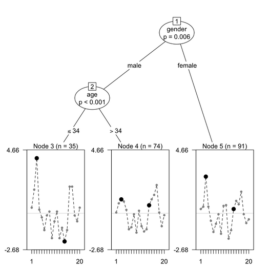
The items that are highlighted in black exhibit DIF. More to say later on.

Computer Adaptive Testing

There’s now the catR package (D. Magis and G. Raiche) for playing with CAT experiments. I didn’t try it yet.

PLS path modeling

I am familiar with the RGCCA and plspm packages for generalized CCA, regularized PLS and PLS path modeling, but now I discovered that there is also semPLS (A. Monecke).

Let’s compare their respective output to a common dataset, namely the mobi data, which comes from a European customer satisfaction index (ECSI) adapted to the mobile phone market, see Tenenhaus et al.⁽²⁾.

Applying the model is as simple as

library(semPLS)
data(ECSImobi)
ecsi <- sempls(model=ECSImobi, data=mobi, E="C")
ecsi

The ECSImobi structure is a convenient wrapper holding the structural and measurement models, which I roughly show below as incidence matrices:

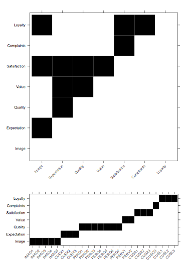
The figures were generated using lattice, as shown below:

levelplot(ECSImobi$M, cuts=1, col.regions=c("white","black"), 
          xlab="", ylab="", colorkey=FALSE, 
          scales=list(x=list(rot=45)))

(Idem for ECSImobi$M.)

There are a lot of outputs, among which we find

• the loadings and path coefficients (LV <-> MV and LV <-> LV) in ecsi$coefficients, which is a summary of ecsi$outer_loadings and ecsi$path_coefficients or ecsi$inner_weights;
• the cross-loadings (all MV <-> LV laodings) are in ecsi$cross_loadings;
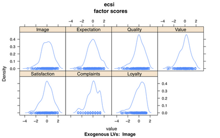
• the factor scores in ecsi$factor_scores: this a 250 by 7 matrix of individual scores for each LV.

We can plot the factor scores using densityplot(ecsi):

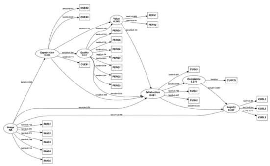
Another very handy function is pathDiagram() which produces a Graphviz file for the PLS path model. Here is how it looks with default settings:

An equivalent formulation of this model using plspm looks like the one provided in the on-line help, with a different model specification:

library(plspm)
data(satisfaction)
IMAG <- c(0,0,0,0,0,0)
EXPE <- c(1,0,0,0,0,0)
QUAL <- c(0,1,0,0,0,0)
VAL  <- c(0,1,1,0,0,0)
SAT  <- c(1,1,1,1,0,0) 
LOY  <- c(1,0,0,0,1,0)
sat.inner <- rbind(IMAG, EXPE, QUAL, VAL, SAT, LOY)
sat.outer <- list(1:5,6:10,11:15,16:19,20:23,24:27)
sat.mod <- rep("A",6)   ## reflective indicators
res2 <- plspm(satisfaction, sat.inner, sat.outer, sat.mod, 
              scaled=FALSE, boot.val=FALSE)
summary(res2)
plot(res2)

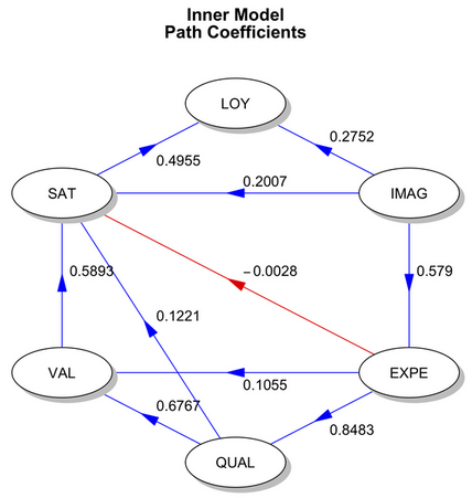
Again, there are useful plot methods, including the one used here to summarize the inner model (which reflects the magnitude of the links between the 6 LVs).

Finally, we could also directly use the lavaan or sem package and fit a traditional CFA/SEM model. In the latter case, there’s also a convenient function called plsm2sem() that allows to convert a plsm object to an object of class mod for usage with interfacing with sem methods.

Network approach

The qgraph package, which I already pointed to in an earlier post, Psychometrics, measurement, and diagnostic medicine.

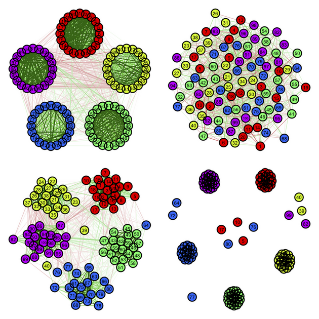
In particular, there are nice illustrations on the Big Five theory of personality traits, as measured by the NEOPI, on the dedicated website. Here is the example I like best, for analyzing correlation matrices, which basically show (1) an association graph with circular or (2) spring layout, (3) a concentration graph with spring layout, and (4) a factorial graph with spring layout (but see help(qgraph.panel)):

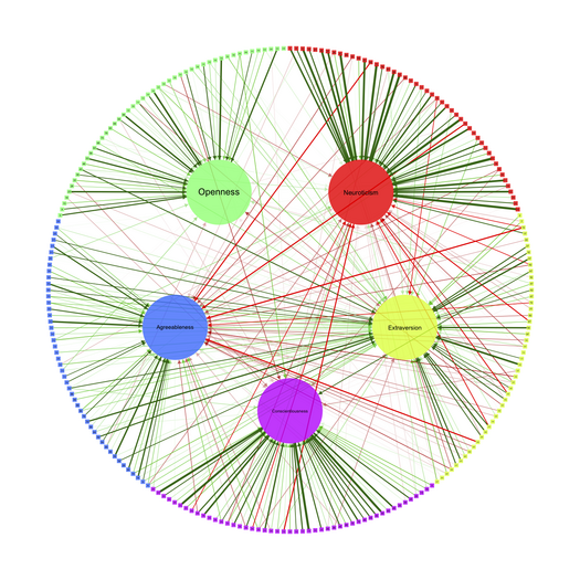
And here is an example for summarizing a standard PCA applied on the NEOPI (see help(qgraph.pca)):

Polytomous items

Although I didn’t found any specific topic around IRT models for polytomous items, I recently tried the ordinal package. The clmm() function allows to fit an ordered logit model with a random intercept, which is also known as a proportional odds model, following McCullagh’s terminology⁽³⁾ (but see Agresti, CDA 2002, pp. 275-277, or Liu and Agresti⁽⁴⁾). Only a single random term is allowed in the current version, but there’s a development package on R-Forge (ordinal2) that might provide extended facilities.

From the on-line help, let’s try to fit a simple model to the soup data, where respondents were asked to rate sample products on an ordered scale with six categories given by combinations of (reference, not reference) and (sure, not sure, guess), in an A-not A discrimination test. Before that, here is a quick view of the individual data (10 responses per subject, N=24 subjects, two types of stimuli):

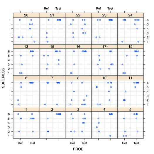
The plot was generated as follows:

library(lattice)
xyplot(SURENESS ~ PROD | RESP, data=dat, type=c("p","g"),
       col=rgb(0,0,1,.5), pch=19,
       panel=function(x, y, ...) { 
         panel.xyplot(jitter(as.numeric(x)), y,...)
       })

Now, our model reads

library(ordinal)
options(contrasts = c("contr.treatment", "contr.poly"))
data(soup)
dat <- subset(soup, as.numeric(as.character(RESP)) <=  24)
dat$RESP <- dat$RESP[drop=TRUE]
m1 <- clmm(SURENESS ~ PROD, random=RESP, data=dat, link="probit",
           Hess=TRUE, method="ucminf", threshold="symmetric")
m1
summary(m1)

The results indicate a signifiant difference between the test and reference products, but also that this model performs better than a reduced (intercept-only) model

anova(m1, update(m1, location=SURENESS ~ 1, Hess=FALSE))

What does this model actually do in practical terms?

Such models are not available in lme4 at the moment, but we could use any IRT model that allows to cope with polytomous items. I should provide an example (e.g. with LPCM() from the eRm package?).

References

1. Zeileis, A. and Hornik, K. (2007). Generalized M-Fluctuation Tests for Parameter Instability. Statistica Neerlandica, 61(4), 488–508.
2. Tenenhaus, M., Vinzi, V.E., Chatelin, Y.-M. and Lauro, C. (2005). PLS path modeling. Computational Statistics & Data Analysis, 48, 159-205.
3. McCullagh, P. (1980). Regression models for ordinal data. Journal of the Royal Society, Series B, 42, 109-142.
4. Liu, I. and Agresti, A. (2005). The analysis of ordered categorical data: An overview and a survey of recent developments. Sociedad de Estadística e Investigación Operativa, 15(1), 1-73.