Phylogenetic trees are used to visually depict the evolutionary relationships between a set of taxa. The branching pattern of such trees is called the topology of the tree, and an interesting question is: What statistcal measure can be used to compare the layout of different evolutionary trees, or in other words, to assess whether their topologies could be considered different? It turns out that the Robinson-Foulds (R-F) distance is exactly what we need, and it is available in the phangorn R package. Besides, this package allows to build trees using different methods, several models of molecular evolution, and to compute their likelihood.

Let’s see it in action. We will use a multi-fasta file containing aligned sequence of different species, from TreeBase. In this case, the dataset consists in 40 sequences of fungi analyzed in the following study: Untereiner W., & Naveaeu F. 1999. Molecular systematics of the Herpotrichiellaceae with an assessment of the phylogenetic positions of Exophiala dermatitidis and Phialophora americana. Mycologia, 91(1): 67-83. Since the data file is already in Nexus format, it is straightforward to import it in R:¹

library("phangorn")
d = read.phyDat("~/tmp/M2043.nex", format = "nexus")
dm = dist.ml(d)
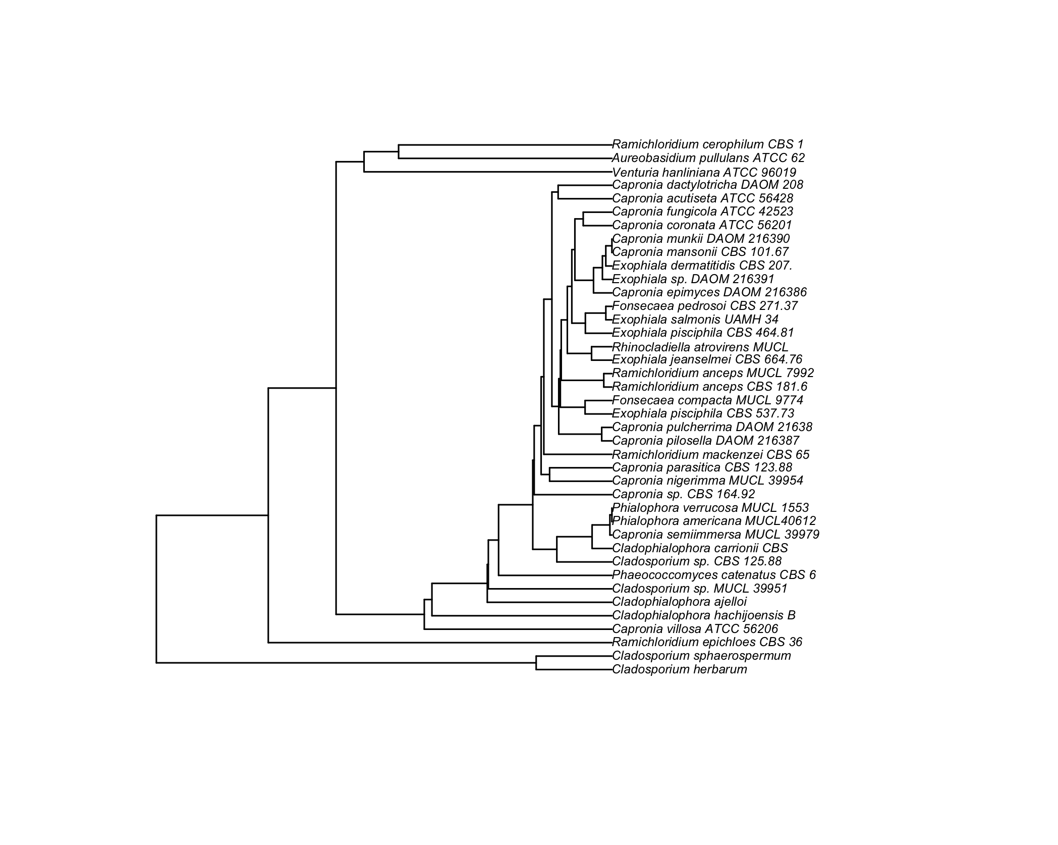
plot(upgma(dm), cex = .5)

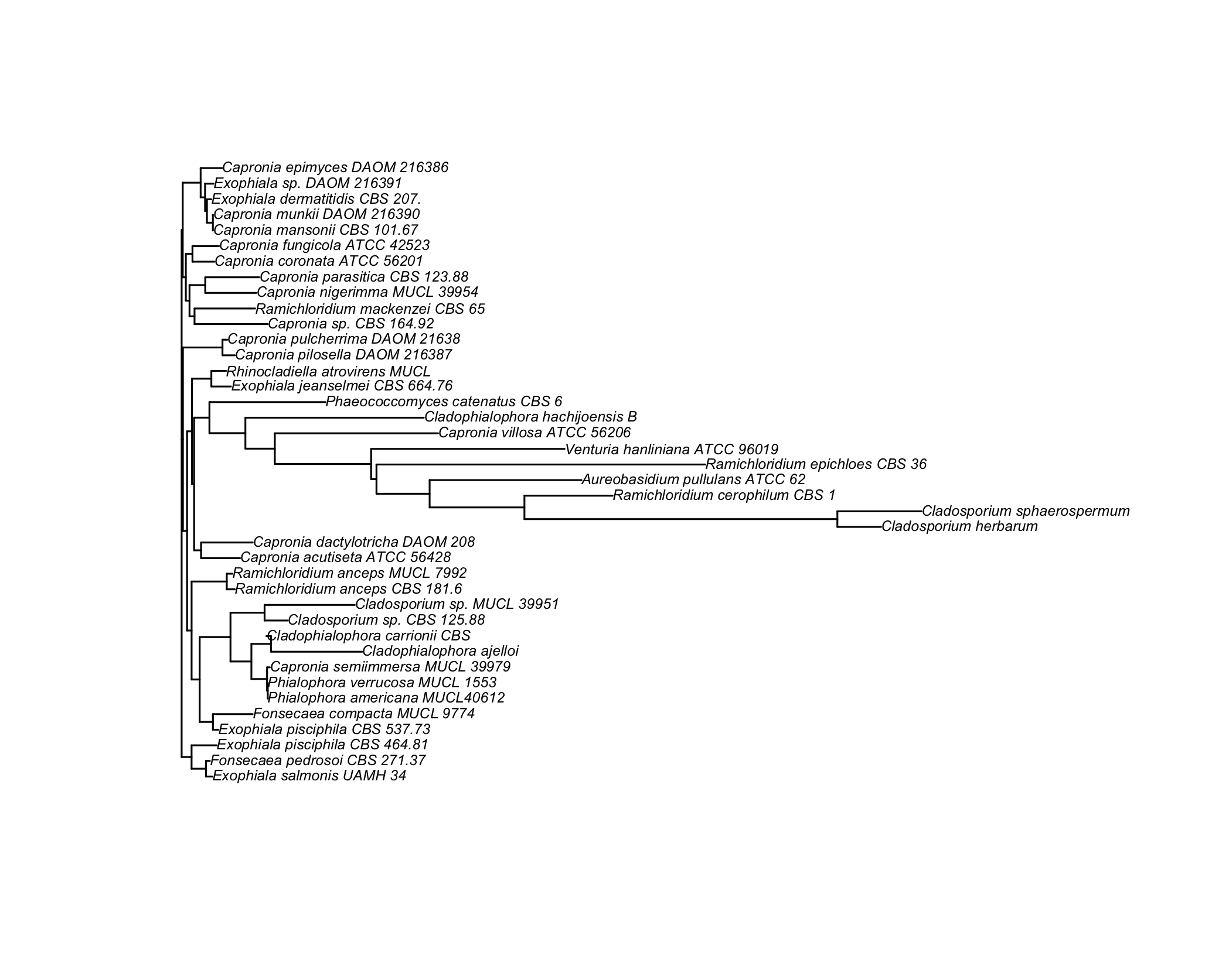
Here are the results of building a tree using unweighted pair group method with arithmetic mean (UPGMA, left) and neighbor joining (NJ, right):

Unrooted trees can be produces as easily by adding the "unrooted" option to the plot function. We could also plot a subset of the whole set of taxa by (approximately) sampling randomly among the common prefix of the taxa, as shown below:

prefix = unlist(lapply(strsplit(names(d), "_"), function(x) x[1]))
idx = seq(1, length(prefix), by = 2)
table(prefix[idx])
d1 = d[idx]
d2 = d[-idx]
dm1 = dist.ml(d1)
dm2 = dist.ml(d2)
op = par(mfrow = c(1, 2), cex = .7)
plot(upgma(dm1))
plot(upgma(dm2))
par(op)

How about using the R-F distance to compare two trees?

tree1 = upgma(dm)
tree2 = NJ(dm)
treedist(tree1, tree2)

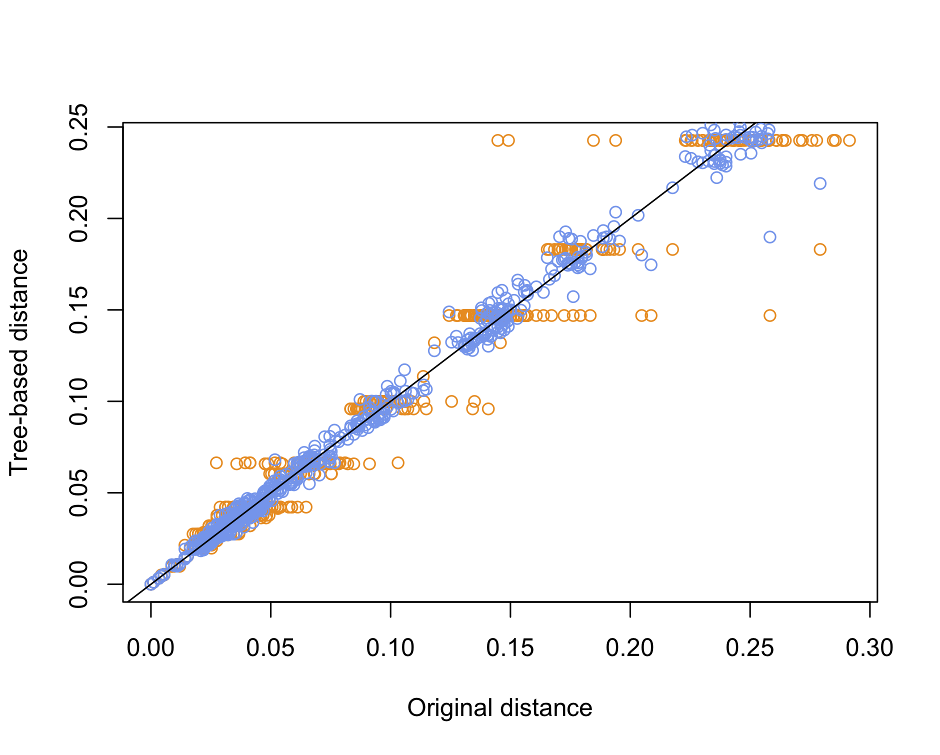
Yet, a simpler approach would be to use the cophenetic distance to compare the original distance with the distance of the species on the tree, whether it is based on NJ or UPGMA. This is basically what we did a long time ago when discussing the quality of clustering methods. Here is an example of use:

dd0 = as.vector(dm)
dd1 = as.vector(as.dist(cophenetic(upgma(dm))))
dd2 = as.vector(as.dist(cophenetic(NJ(dm))))
plot(dd0, dd1, col = "darkorange", xlab = "Original distance", ylab = "Tree-based distance")
points(dd0, dd2, col = "cornflowerblue")
abline(0, 1)

We can conclude that the NJ method offers the best reconstruction of the original pairwise distance matrix, which is to be expected since UPGMA imposes an ultrametric property whereby all tips should be equidistant from the root, which is another way to say that all species have undergone the same amount of evolution.

Finally, to compute the likelihood of those trees, we can re-use the omnibus anova function, as we would do for comparing two statistical models:

m1 = pml(upgma(dm), data = d)
m2 = pml(NJ(dm), data = d)
anova(m1, m2)
logLik(m2)

In the case of the NJ tree I got a log likelihood of -6526.059, with 77 degrees of freedom. Instead of this base model, we could consider the Jukes-Cantor model we discussed earlier:

m.jc = optim.pml(m, optNni = TRUE)
logLik(m.jc)  # 'log Lik.' -6451.672 (df=77)

Where do these degrees of freedom come from and how do we define the likelihood of a tree after all? Of course, the likelihood here stands for the probability that such a tree would have generated the data presented in the sequence under the chosen model. If we make the assumption that each site evolves independently, we can compute separately the likelihood at each site and add them up. For each site, its likelihood is defined as the sum of the probabilities of every possible ancestral states, which conform to the Jukes-Cantor substitution model (equiprobable substitutions and equiprobable base frequencies). Basically, this amounts to compute conditional likelihood (starting from the tip of the tree down to the common ancestral root). It can be shown that for any node $x$, whose immediate descendants are tips $y$ and $z$, the conditional likelihood at node $k$ amounts to:

$$ L_S^{(x)} = \sum_s \left[ \left(\sum_{S_y} P_{S_xS_y}(v_y)L_{S_y}^{(y)} \right) \left(\sum_{S_z} P_{S_xS_z}(v_z)L_{S_z}^{(z)} \right) \right]. $$

These conditional likelihoods are computed iteratively from the tips to the root of the tree. Once we get the conditional likelihood $L_{S_0}^0$ for the root (0), the overall likelihood is just the sum of all those conditional likelihoods:

$$ \mathcal{L} = \sum_{S_{0}} \pi_{S_0}L_{S_0}^{(0)}, $$

where $\pi_{S_0}$ denotes the base frequencies for the root of the tree, that is the probability that the root is in state $S_{0}$. Of course, every model comes with its own set of hyperparameters (e.g., the GTR adds 4 four parameters), hence the varying amount of degrees of freedom that we can find from one model to the other. There’s also a nice discussion of on the following blog post: Likelihood of a tree.